Reading time 8 minutes

KZNF protein pathway regulation

24 June 2022

Exec summary
Background
- Typical approach
- New approach
Case study
- Protocol
- Result
Summary
Code used
References

Exec summary

We use existing data to show an improved method for identifying ZNF-dependent gene regulation at the:
1. gene level.
2. protein pathway level.
The method is statistically unbiased and might be used to produce more successful functional validation studies.

I will go thorough the steps to get to this final summary image:

Background

Control of gene expression by KZNFs occurs throughout the genome.
Clusters of several genes within a single region are affected by one KZNF binding site.
Research often focuses on one KZNF at a time
- functional experiment require a ZNF in vitro system and Chip-seq
Research often focuses on the resulting best candidate:
- a single genome site that had the larges change in expression
- to top gene in that region (for whatever reason)
- nearst gene to the regulotory region

ZNF genes that are intolerant to LoF (pLI = 1) are very interesting:
- since their function is regulation of expression for target genes
- the targets themselves must also have a intollerance to LoF
ZNF targets can be many gene (i) genome wide (ii) clustered together.
Genome-wide ZNF targets might form a protein pathway
pLI ZNF targets may also be (i) individually pLI or (ii) cumulatively pLI for a pathway.

Typical approach

Make a ZNF in vitro assay
Chip-seq
Find genes with DE
Explain the top hit
Or pass all hits into GO for a pathway report.

Opinion:

Result #4 is interesting and requires a lot of functional work.
Result #5 is generally not very insightful and often focuses on a cluster of genes, rather than genome-wide.

New approach

Select a pLI ZNF (pilot study)
Make a ZNF in vitro assay
Chip-seq
Find genes with DE
Cluster all target genes into their protein pathways
Identify pathways where all genes are (i) individually pLI or (ii) cumulatively pLI for the pathway.

Opinion:

This result unbiased for picking what you determine to be the “top hit”.
The mechanisms of pLI (and therefore ZFN downstream effect) can be interpreted from existing evidence
- for all genes withing the pathway, functional explanation is likely avaiable (Uniprot + GTEx)
A successful pilot in the most damaging pLI will provide a route to more complex and subtle regulatory mechanisms
- i.e. genes/pathways that are tollerant to haploinsuffiency which would otherwise be at the mercy of blind functional analysis.

Case study

Protocol

0. Select a pLI ZNF (pilot study)

The closer pLI is to one, the more intolerant of protein-truncating variants the transcript appears to be. We consider pLI ≥ 0.9 as an extremely intolerant set of transcripts. (Lek et al., 2016).

Methods in Code block 1

To find ZNF genes with pLI >0.9 I used

https://gnomad.broadinstitute.org/downloads
Section “Constraint”
File “pLoF Metrics by Gene TSV”
Ref https://www.nature.com/articles/s41586-020-2308-7
(Lek et al., 2016).

Handling requires installation of samtools https://www.htslib.org (Samtools, BCFtools, HTSlib). Uncompress the data with bgzip.

Methods in Code block 2

Query the whole genoe pLI score for all ZNF genes. Clean the dataset to extract the data of interest: Gene name, numbers of observed/expected LoF, pLI score, etc.

Methods in Code block 3

The R code performs a lot of formatting and cleaning to interpret the dataset. We find all genes wiht pLI > 0.9.

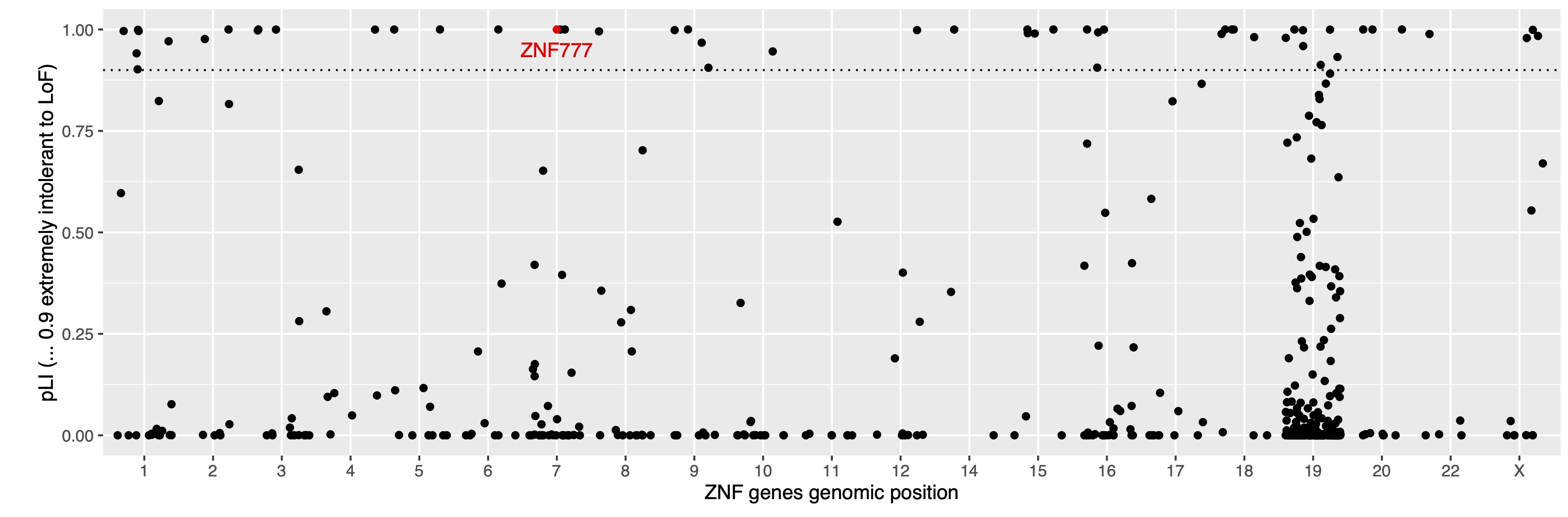
I have pre-emptively shown ZNF777 in red. I will show in the next section why I chose this as a pilot study.

1. Make a ZNF in vitro assay

This was found from existing data, as shown in the next section.

2. Chip-seq

This was found from existing data, as shown in the next section.

3. Find genes with DE

I used existing chip-seq data. This will pair one ZNF to a list of all genes that it ostensibly regulates. I believe this dataset to be a useful example: (Imbeault et al., 2017), https://www.nature.com/articles/nature21683.

“We then determined the genomic targets of human KZFPs by performing chromatin immunoprecipitation with exonuclease digestion (ChIP–exo)[13] on 257 HEK293T cell lines, each engineered to express one haemagglutinin (HA)-tagged family member. We obtained single base-pair resolution binding sites for 222 human KZFPs (Supplementary Table 4), 12 of them in duplicate (Extended Data Fig. 2), with the number of high-quality peaks per protein ranging from more than 10,000 to only around 15 (Extended Data Fig. 3a).

I compared my list of all ZNF for pLI >0.9 with the ZNF genes available in this study. The first match was ZNF777, which has pLI 0.99 (as shown in Figure 1).

I downloaded the data:

GSM2466654 ZNF777 -https://www.ncbi.nlm.nih.gov/geo/query/acc.cgi?acc=GSE78099 -https://www.ncbi.nlm.nih.gov/geo/query/acc.cgi?acc=GSM2466654
Methods in Code block 3

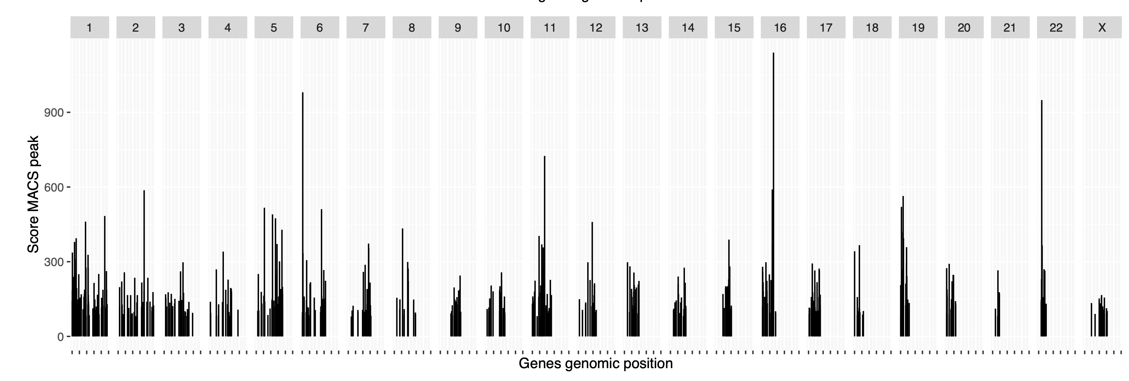
I cleaned and visualise the MACS (Model-based Analysis of ChIP-Seq) peak data. What is MACS? - ref 1, (Feng et al., 2011). What is MACS? - ref 2

4. Cluster all target genes into their protein pathways

Methods in Code block 4
Methods in Code block 5
Methods in Code block 6 (The data contained genomic coordinates so I needed to gene coding region protein for further steps.)
Methods in Code block 3

The genes “affected” by ZNF777 were clustered into their best-fit protein pathways using STRING-db. String uses experimental and curated data from Biocarta, BioCyc, GO, KEGG, and Reactome, BIND, DIP, GRID, HPRD, IntAct, MINT, and PID.

I access the database using Cytoscape.

Pathway clustering was performed using Markov Cluster Algorithm (MCL), an unsupervised cluster algorithm for networks based on stochastic flow. (Van Dongen, 2000), https://micans.org/mcl/.

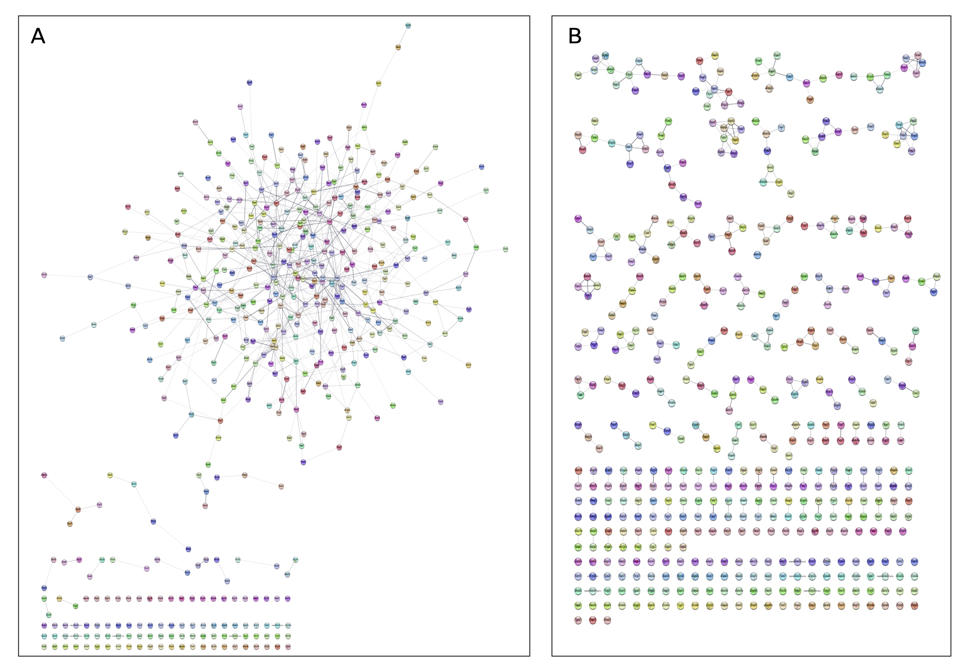
In Figure A, I show all of the gene target of ZNF777.

Each node illustrates one protein.
Each edge illustrates the weight of evidence connecting proteins.

Since we cannot define the protein pathways clearly here (something that you find when reading hierarchical GO enrichement analsis results), I instead cluster these proteins into the best-fitting pathways.

The result of MCL clustering is show in Figure B.

Now we have a set of distinct protein pathways.

5. Identify pathways with pLI

Methods in Code block 3

Next, since we started with a ZNF that is intolerant to LoF, we also believe that the target genes must also be

(i) individually pLI
or (ii) cumulatively pLI for the pathway.

I cleaned the data further to group gene according to their

protein pathways,
genomic distribution, and
pLI score.

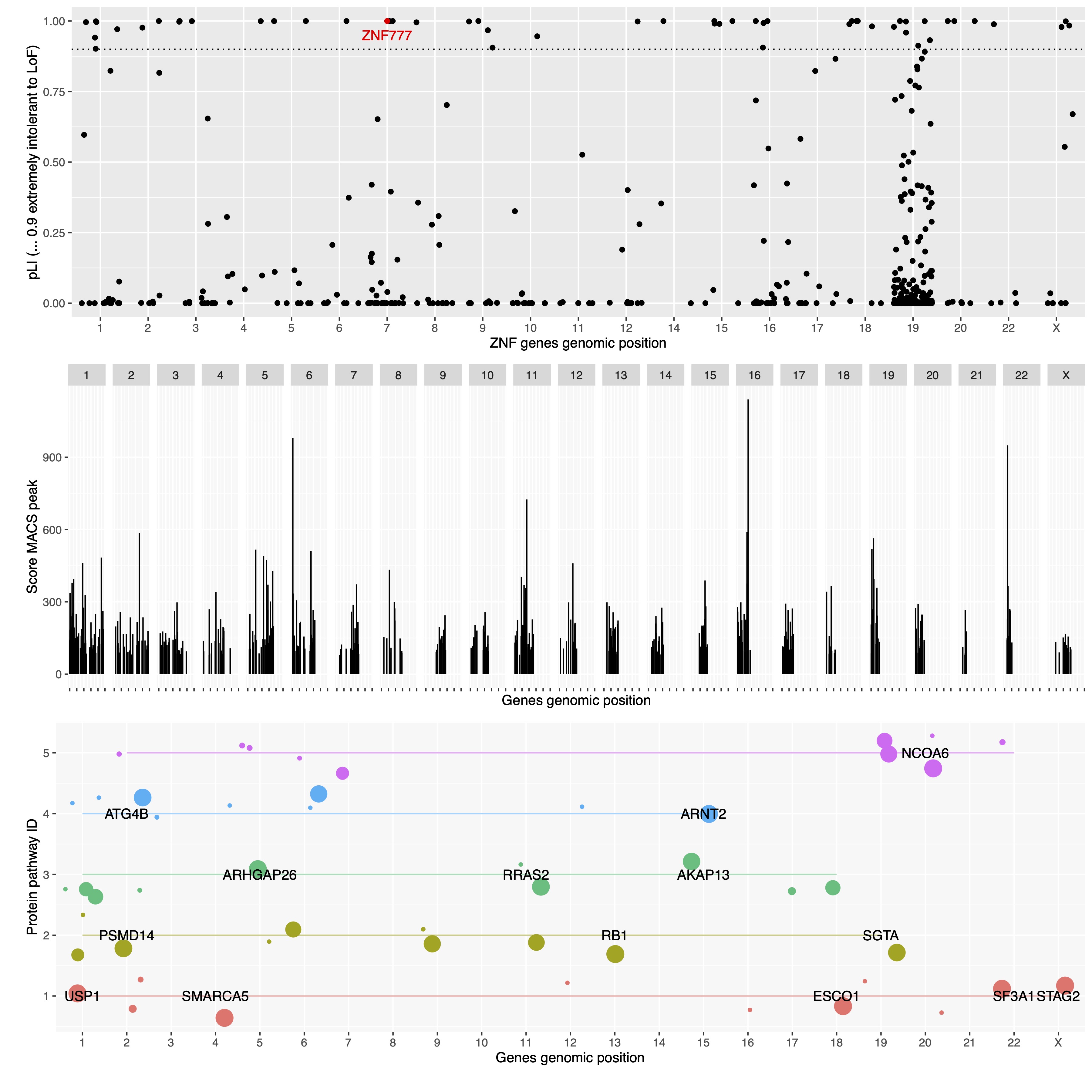
Figure 3 shows the top 5 largest pathways.

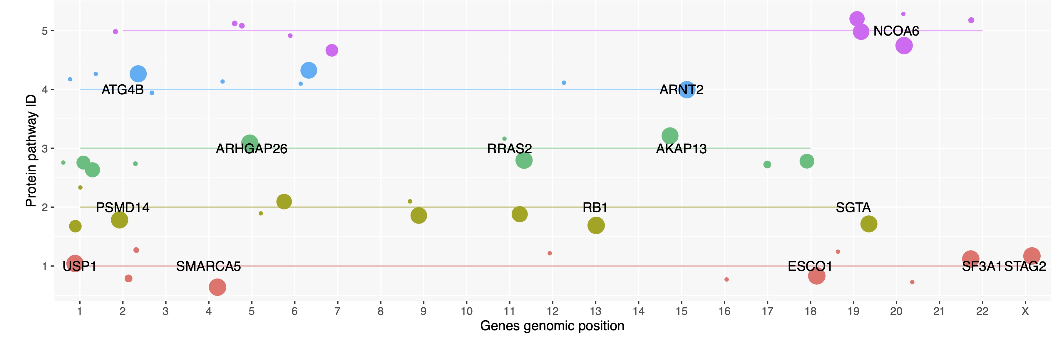
Key: We can see that rahter than focusing on a cluster of genes within one genomic region, we interpret genes according to their protein pthway.
Some protein pathways will have high pLI scores and may be considered the major ZNF targets.
Some protein pathways can tolerate LoF and maybe considered by-standers.

These by-stander genes are still surely sensitive to regulation by ZNF777. However, we can infer the evolutionary hierarchy of the major and minor protein pathways under the control of this ZNF.

6. Further development

There are 2 major further ways to progress.

Complete all avaialble Chip-seq datasets for pLI >0.9. Expand into pLI below 0.9 if possible.
Find which genes are in these protein pathways and see why they are not regulated by this ZNF (and see if there are sister ZNFs working in tangent to control pathway dosages).

Result

From all candidate ZNF gene targets, we find those which match it’s intolerance to LoF. We therefore define these pathways as the major targets of this ZNF.

I have purposely refrained for completing the final step: quantifying the top pLI pathway/gene list. This is to prevent from making a conclusion without testing the theory and stats.

Summary

Code used

1.unzip.sh

#!/bin/bash

# dataset
# <https://gnomad.broadinstitute.org/downloads>
# Section "Constraint"
# File "pLoF Metrics by Gene TSV"
# Ref <https://www.nature.com/articles/s41586-020-2308-7>

# install samtools

bgzip -d gnomad.v2.1.1.lof_metrics.by_gene.txt.bgz

2.scan.sh

#!/bin/bash
set -e
cd ../data/

output=ZNF_summary.tsv

# query gene and get summary column
head -1 gnomad.v2.1.1.lof_metrics.by_gene.txt | cut -f 1,17,18,20,21,42,43,46,75,76,77 > $output
# obs_lof	mu_lof	exp_lof	pLI	obs_het_lof	obs_hom_lof	exp_hom_lof

grep "ZNF*" gnomad.v2.1.1.lof_metrics.by_gene.txt | cut -f 1,17,18,20,21,42,43,46,75,76,77 >> $output

3.analyse.R

Major note: some of the data used in the second half of this script requires the scripts from 4,5,6. I have named them in the order of writing. It will be obvious when a dataset is missing, that the next bash script should be run. If continuing this project, 3.analyse.R should be split into sequential order, or call the bash script within the R code.

Minor note: This script is needlessly long and contains rough exploration work. If continuing this project, it can be heavily simplified.

library(dplyr)
library(ggplot2)
library(tidyr)

# Multiple sequence alignment file
df <- 
	read.table(file="../data/ZNF_summary.tsv", 
				  header = TRUE, 
				  sep = "\t", 
				  stringsAsFactors = FALSE)

# Note there is one KAZN gene included, figure out the grep correction later.

# The closer pLI is to one, the more intolerant of protein-truncating variants the transcript appears to be. We consider pLI ≥ 0.9 as an extremely intolerant set of transcripts. _Lek et al Nature 2016._
names(df)

# get the data in chr order
df <- arrange(df, chromosome, start_position)

df$chromosome <- as.numeric(df$chromosome)
df$start_position <- as.numeric(df$start_position)

# replace NAs with X chromosome 
df$chromosome[is.na(df$chromosome)]<-"X"

# create the subset for example: ZNF777
g1 <- subset(df, gene == "ZNF777")

pZNF777 <- 
	df %>%
#	ggplot(aes(x=start_position, y=pLI))+
	ggplot(aes(x=factor(chromosome, stringr::str_sort(unique(chromosome), numeric = TRUE)),
				  y=pLI))+
#	geom_point() +
	geom_jitter() +
	geom_point(data=g1, colour="red") +  # this adds a red point
	geom_text(data=g1, label="ZNF777", y=.95, colour="red") +
	geom_hline(linetype="dotted", yintercept=0.9) +
	#facet_grid(~chromosome) +
#	facet_grid(.~factor(chromosome, stringr::str_sort(unique(chromosome), numeric = TRUE))) + 
#	theme(legend.position="none", panel.background = element_rect("#F7F7F7"),
#			#axis.text.x=element_text(angle=45,hjust=1,vjust=0.5),
#			axis.text.x=element_blank()) +
	xlab("ZNF genes genomic position") +
	ylab("pLI (≥ 0.9 extremely intolerant to LoF)") 

pZNF777

# Next I want to simulate some chip-seq data, matching one ZNF to a list of all genes that are regulated
# I believe this dataset is useful
#### https://www.nature.com/articles/nature21683
# We then determined the genomic targets of human KZFPs by performing chromatin immunoprecipitation with exonuclease digestion (ChIP–exo)13 on 257 HEK293T cell lines, each engineered to express one haemagglutinin (HA)-tagged family member. We obtained single base-pair resolution binding sites for 222 human KZFPs (Supplementary Table 4), 12 of them in duplicate (Extended Data Fig. 2), with the number of high-quality peaks per protein ranging from more than 10,000 to only around 15 (Extended Data Fig. 3a). 

#ZNF77 has pLI 0.99
# Download
# GSM2466654	ZNF777
# https://www.ncbi.nlm.nih.gov/geo/query/acc.cgi?acc=GSE78099
## https://www.ncbi.nlm.nih.gov/geo/query/acc.cgi?acc=GSM2466654

df2 <- 
	read.table(file="../data/GSM2466654_ZNF777_peaks_processed_score_signal_exo.bed.txt", 
				  header = FALSE, 
				  sep = "\t", 
				  stringsAsFactors = FALSE)

df2 <- separate(df2, V1, into = c("text", "chromosome"), sep = "chr") %>% select(-text)

colnames(df2)[colnames(df2) == 'V2'] <- 'start_position'
colnames(df2)[colnames(df2) == 'V3'] <- 'end_position'
colnames(df2)[colnames(df2) == 'V5'] <- 'score'

df2 %>%
	ggplot(aes(x=start_position, y=score ))+
	geom_point() +
#	geom_hline(linetype="dotted", yintercept=0.9) +
	#facet_grid(~chromosome) +
	facet_grid(.~factor(chromosome, stringr::str_sort(unique(chromosome), numeric = TRUE))) + 
	theme(legend.position="none", panel.background = element_rect("#F7F7F7"),
			#axis.text.x=element_text(angle=45,hjust=1,vjust=0.5),
			axis.text.x=element_blank()) +
	xlab("Genes genomic position") +
	ylab("Score MACS peak") 

# aligned to GRCh37g1k 

# get gene symbtols via ensenbke biomart
# http://grch37.ensembl.org/biomart/martview/35883cadc275e8738b07668ab1f8d58f

# run 4.chip.sh

# Query for these coordinates and output attibutes:
#Dataset : Human genes (GRCh37.p13)
#Filters: coordinates, e.g. 1:100:10000:-1, 1:100000:200000:1: [ID-list specified]
#Attributes:
#Gene stable ID
#Gene start (bp)
#Gene end (bp)
#Chromosome/scaffold name
#Transcription start site (TSS)
#Gene name

# Output: GSM2466654_ZNF777_peaks_processed_score_signal_exo.bed.biomartformat_annotated.txt

df3 <- 
	read.table(file="../data/GSM2466654_ZNF777_peaks_processed_score_signal_exo.bed.biomartformat_annotated.txt", 
				  header = TRUE, 
				  sep = "\t", 
				  stringsAsFactors = FALSE)

# run 5.genelist.sh

# cytoscape 
# string gene query, print list
# MCL cluster, default 2.5 inflation

df4 <- 
	read.table(file="../output/img2_string_network_ZNF777_peaks_MCL2.5_table.csv", 
				  header = TRUE, 
				  sep = ",", 
				  stringsAsFactors = FALSE)

df4 <- df4 %>% select(X__mclCluster, display.name) 

# colnames(df)[colnames(df) == 'oldName'] <- 'newName'
colnames(df4)[colnames(df4) == 'display.name'] <- 'Gene.name'
colnames(df4)[colnames(df4) == 'X__mclCluster'] <- 'mclCluster'

# merge MCL clusters with the MACS peaks (genes named via biomart)
df5 <- merge(df3, df4)

# get first in gene (instead of all TSS)
df5 <- df5 %>%
	group_by(Gene.name) %>%
	filter(row_number()==1)

names(df5)

colnames(df5)[colnames(df5) == 'Chromosome.scaffold.name'] <- 'chromosome'
colnames(df5)[colnames(df5) == 'Gene.start..bp.'] <- 'start_position'
colnames(df5)[colnames(df5) == 'Gene.end..bp.'] <- 'end_position'

df5 %>%
	ggplot(aes(x=start_position, y=(mclCluster), color= (as.character(mclCluster) ) ))+
	geom_point() +
	#	geom_hline(linetype="dotted", yintercept=0.9) +
	#facet_grid(~chromosome) +
	facet_grid(~factor(chromosome, stringr::str_sort(unique(chromosome), numeric = TRUE))) + 
	theme(legend.position="none", panel.background = element_rect("#F7F7F7"),
			#axis.text.x=element_text(angle=45,hjust=1,vjust=0.5),
			axis.text.x=element_blank()) +
	xlab("Genes genomic position") +
	ylab("Score MACS peak") 


df5 %>%
	ggplot(aes(x=factor(chromosome, stringr::str_sort(unique(chromosome), numeric = TRUE)), 
				  y=(mclCluster), 
				  group=mclCluster,
				  color= (as.character(mclCluster) ) ))+
	#geom_point() +
	geom_jitter() +
	geom_line(aes(alpha=0.2)) +
	theme(legend.position="none", panel.background = element_rect("#F7F7F7"),
			#axis.text.x=element_text(angle=45,hjust=1,vjust=0.5),
			#axis.text.x=element_blank()
			) +
	xlab("Genes genomic position") +
	ylab("Protein pathway ID") 

# merge protein pathway data with MACS peaks

df5 <- df5 %>% filter(mclCluster < 6)

df2
names(df2)
names(df5)

tmp <- merge(
	(df2 %>% select(chromosome, start_position, end_position, score)),
	(df5 %>% select(Gene.name, chromosome, start_position, end_position, mclCluster)),
	all = T )

df2 <- df2 %>% 
	select(chromosome, start_position, end_position, score)

tmp <- merge(df2, df5, all = T )

# get pLI scores
# now get the plof for mcl genes
gene_names <- tmp %>% filter(mclCluster > 0) %>% select(Gene.name)

write.table(gene_names, file='../output/gene_names_mcl_top5.csv',sep=",", quote=FALSE, row.names=FALSE, col.names = FALSE)

# run 6.mclplof.sh

# Multiple sequence alignment file
df6 <- 
	read.table(file="../output/gene_names_mcl_top5_plof.txt", 
				  header = TRUE, 
				  sep = "\t", 
				  stringsAsFactors = FALSE)

names(tmp)
names(df6)

# colnames(df6)[colnames(df6) == 'oldName'] <- 'newName'
colnames(df6)[colnames(df6) == 'gene'] <- 'Gene.name'

tmp <- merge(tmp, df6, all.x = T)

tmp %>%
	ggplot(aes(x=factor(chromosome, stringr::str_sort(unique(chromosome), numeric = TRUE)), 
				  y=mclCluster, 
				  group=mclCluster,
				  color= (as.character(mclCluster) ) ))+
#	geom_point() +
	geom_jitter() +
	geom_line(aes(alpha=0.2)) +
	theme(legend.position="none", panel.background = element_rect("#F7F7F7"),
			#axis.text.x=element_text(angle=45,hjust=1,vjust=0.5),
			#axis.text.x=element_blank()
	) +
	xlab("Genes genomic position") +
	ylab("Protein pathway ID") 

p0 <- tmp %>%
#	filter(chromosome ==1 ) %>%
	ggplot(aes(x=start_position, 
				  y=mclCluster, 
				  group=mclCluster,
				  color= (as.character(mclCluster) ) ))+
#	geom_point() +
	geom_jitter() +
	geom_line(aes(alpha=0.2)) +
	theme(legend.position="none", panel.background = element_rect("#F7F7F7"),
			#axis.text.x=element_text(angle=45,hjust=1,vjust=0.5),
			#axis.text.x=element_blank()
	) +
	xlab("Genes genomic position") +
	ylab("Protein pathway ID") 

g2$Gene.name
g2 <- subset(tmp, pLI >= 0.9)
p1 <- tmp2 %>%
	ggplot(aes(x=factor(chromosome, stringr::str_sort(unique(chromosome), numeric = TRUE)), 
				  y=(mclCluster), 
				  group=mclCluster,
				  color= (as.character(mclCluster) ) ))+
	#geom_point() +
	geom_jitter(aes(size=pLI)) +
	geom_line(aes(alpha=0.2)) +
	theme(legend.position="none", panel.background = element_rect("#F7F7F7"),
			#axis.text.x=element_text(angle=45,hjust=1,vjust=0.5),
			#axis.text.x=element_blank()
	) +
	xlab("Genes genomic position") +
	ylab("Protein pathway ID")  + 
	geom_text(data=g2, aes(label=Gene.name), color='black')

p2 <- tmp %>%
#	filter(chromosome ==1 ) %>%
	ggplot(aes(start_position, score ))+
	geom_segment(aes(xend = start_position, yend = 0))+
	facet_grid(.~factor(chromosome, stringr::str_sort(unique(chromosome), numeric = TRUE))) +
	theme(legend.position="none", panel.background = element_rect("#F7F7F7"),
			#axis.text.x=element_text(angle=45,hjust=1,vjust=0.5),
			axis.text.x=element_blank()) +
	xlab("Genes genomic position") +
	ylab("Score MACS peak") 

# Plot main figure ----
require(gridExtra)
grid.arrange(pZNF777, p2, p1,ncol=1, 
				 bottom = "", 
				 left = "") 

4.chip.sh

#!/bin/bash

cd ../data/

# convert to correct format
# (Chr:Start:End:Strand) [Max 500 advised]
# e.g. 1:100:10000:-1, 1:100000:200000:1

cut -f 1-3 GSM2466654_ZNF777_peaks_processed_score_signal_exo.bed.txt |\
	sed 's/	/:/g' |\
	sed 's/chr//g' \
	> GSM2466654_ZNF777_peaks_processed_score_signal_exo.bed.biomartformat.txt

5.genelist.sh

#!/bin/bash

# gene simple gene list to cluster with STRING
cut -f 6 GSM2466654_ZNF777_peaks_processed_score_signal_exo.bed.biomartformat_annotated.txt |\
	sort |\
	uniq \
	> GSM2466654_ZNF777_peaks_processed_score_signal_exo.bed.biomartformat_annotated_genes.txt

6.mclplof.sh

#!/bin/bash
cd ../output/

# for every line in the top 5 protein pathways, get the pLI data
head -1 ../data/gnomad.v2.1.1.lof_metrics.by_gene.txt | cut -f 1,17,18,20,21,42,43,46,75,76,77 > gene_names_mcl_top5_plof.txt

while read -r line; 
do 
grep "$line"  ../data/gnomad.v2.1.1.lof_metrics.by_gene.txt;
done < gene_names_mcl_top5.csv  |\
	cut -f 1,17,18,20,21,42,43,46,75,76,77 >> gene_names_mcl_top5_plof.txt

References

Lek, M., Karczewski, K. J., Minikel, E. V., Samocha, K. E., Banks, E., Fennell, T., O’Donnell-Luria, A. H., Ware, J. S., Hill, A. J., Cummings, B. B., & others. (2016). Analysis of protein-coding genetic variation in 60,706 humans. Nature, 536(7616), 285.
Imbeault, M., Helleboid, P.-Y., & Trono, D. (2017). KRAB zinc-finger proteins contribute to the evolution of gene regulatory networks. Nature, 543(7646), 550–554.
Feng, J., Liu, T., & Zhang, Y. (2011). Using MACS to identify peaks from ChIP-Seq data. Current Protocols in Bioinformatics, 34(1), 2–14.
Van Dongen, S. M. (2000). Graph clustering by flow simulation [PhD thesis].