Analysis of methods

• The fianl comparison results
  • Scores per sample and Bland-Altman plot
  • Correlation test result and repeatability coefficients
• Code
• Summary of the analysis of method comparison studies

Altman, D. G., and J. M. Bland. “Measurement in Medicine: The Analysis of Method Comparison Studies.” Journal of the Royal Statistical Society. Series D (The Statistician), vol. 32, no. 3, 1983, pp. 307–17. JSTOR, https://doi.org/10.2307/2987937.

The paper is a pivotal guide discussing the analysis of method comparison studies, particularly in the field of medicine. It proposes a pragmatic approach to analyze such studies, stressing the importance of simplicity especially when the results need to be explained to non-statisticians. I work through it here to compare if a new methods is as good or better than an existing one for clinical sepsis scores with example data.

For more similar papers see the series of BMJ statistical notes by Altman & Bland ( lit-altman_bland.md ).

The fianl comparison results

Scores per sample and Bland-Altman plot

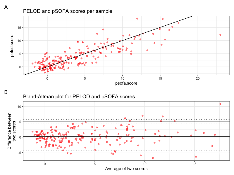Figure 1. Scores per sample and Bland-Altman plot as produced by the provided R code.

Correlation test result and repeatability coefficients

Results of the analysis as produced by the provided R code:

$Repeatability_Score1
[1] 4.674812

$Repeatability_Score2
[1] 4.267645

$Correlation_Test

	Pearson's product-moment correlation

data:  df$score1 and df$score2
t = 21.693, df = 197, p-value < 2.2e-16
alternative hypothesis: true correlation is not equal to 0
95 percent confidence interval:
 0.7931229 0.8763442
sample estimates:
      cor 
0.8395928 

Repeatability Scores:

• Repeatability Score 1: 4.674812
• Repeatability Score 2: 4.267645

The repeatability scores are measures of how consistent each method is. In this case, both methods seem to have fairly similar repeatability scores, indicating a similar level of consistency or reliability within each method. Without context or a benchmark to compare to, it’s challenging to definitively say whether these scores are good or not, but the similarity suggests comparable repeatability.

Correlation Test:

• Pearson’s Correlation Coefficient (r): 0.8395928
• 95% Confidence Interval for r: [0.7931229, 0.8763442]
• P-value: \(< 2.2e-16\)

The Pearson’s correlation coefficient is quite high, indicating a strong positive linear relationship between the scores from the two methods. The nearly zero p-value (less than 2.2e-16) strongly suggests that this correlation is statistically significant, and it’s highly unlikely that this observed correlation occurred by chance.

Conclusion:

Considering the high correlation coefficient and the comparable repeatability scores, it seems that the new method is quite similar to the old one in terms of both reliability (as indicated by the repeatability scores) and agreement (as indicated by the correlation coefficient).

Code

# Here is a really cool set of notes in BMJ about all kinds of clinical data analysis.
# https://www-users.york.ac.uk/~mb55/pubs/pbstnote.htm

# For example, if you every like to go further with the score that you working on, this paper is very famous for showing how to compare two such clinical score methods to show if the new one performs better. 

# https://sci-hub.hkvisa.net/10.2307/2987937
# (Measurement in Medicine: The Analysis of Method Comparison Studies Author(s): D. G. Altman and J. M. Bland 1983)

# Example ----
# psofa.score - Total number of organ failures according to 2017 pSOFA definitions (Matics et al. (2017) (PMID 28783810)). The classification of organ failures is based on the worst vital signs and the worst lab values during the first 7 days from blood culture sampling.

# pelod.score - Total number of organ failures according to PELOD-2 definitions (Leteurtre et al. (2013) (PMID 23685639)). The classification of organ failures is based on the worst vital signs and the worst lab values during the first 7 days from blood culture sampling.

library(ggplot2)
library(dplyr)
library(tidyr)
library(patchwork)

# Read data
df <- read.csv(file = "../data/example_sepsis_scores.tsv", sep = " ")

# Take 200 rows as an example
df <- df[1:200, ]

# Renaming columns and adding index column
df$score1 <- df$psofa.score
df$score2 <- df$pelod.score
df$index <- rownames(df)

# Adding a small amount of random noise to each value
# NOTE: THIS WOULD BE USED FOR ADDING SOME NOISE TO MAKE THE DATA MORE ANONYMOUS FOR PUBLISHING AN EXAMPLE FIGURE
set.seed(123) # Setting a seed to ensure reproducibility
df$score1 <- df$score1 + rnorm(nrow(df), mean = 0, sd = 1)
df$score2 <- df$score2 + rnorm(nrow(df), mean = 0, sd = 1)

# Calculate necessary statistics: the average and the difference of score1 and score2.
df$means <- (df$score1 + df$score2) / 2
df$diffs <- df$score1 - df$score2

# Compute repeatability coefficients for each method separately
repeatability_score1 <- sd(df$score1, na.rm = TRUE)
repeatability_score2 <- sd(df$score2, na.rm = TRUE)

# Compute correlation to check independence of repeatability from the size of the measurements
cor_test <- cor.test(df$score1, df$score2, method = "pearson")

# Average difference (aka the bias)
bias <- mean(df$diffs, na.rm = TRUE) 

# Sample standard deviation
sd <- sd(df$diffs, na.rm = TRUE) 

# Limits of agreement
upper_loa <- bias + 1.96 * sd
lower_loa <- bias - 1.96 * sd

# Additional statistics for confidence intervals
n <- nrow(df)
conf_int <- 0.95
t1 <- qt((1 - conf_int) / 2, df = n - 1)
t2 <- qt((conf_int + 1) / 2, df = n - 1)
var <- sd^2
se_bias <- sqrt(var / n)
se_loas <- sqrt(3 * var / n)
upper_loa_ci_lower <- upper_loa + t1 * se_loas
upper_loa_ci_upper <- upper_loa + t2 * se_loas
bias_ci_lower <- bias + t1 * se_bias
bias_ci_upper <- bias + t2 * se_bias
lower_loa_ci_lower <- lower_loa + t1 * se_loas
lower_loa_ci_upper <- lower_loa + t2 * se_loas

# Create Bland-Altman plot
p1 <- df |>
  ggplot(aes(x = means, y = diffs)) + 
  geom_point(color = "red", alpha = .5) +
  ggtitle("Bland-Altman plot for PELOD and pSOFA scores") + 
  ylab("Difference between\ntwo scores") + 
  xlab("Average of two scores") +
  theme_bw() +
  geom_hline(yintercept = c(lower_loa, bias, upper_loa), linetype = "solid") +
  geom_hline(yintercept = c(lower_loa_ci_lower, lower_loa_ci_upper, upper_loa_ci_lower, upper_loa_ci_upper), linetype="dotted") +
  geom_hline(yintercept = se_bias)

# Create scatter plot with a line of equality
p2 <- df |>
  ggplot(aes(x=score1, y=score2)) +
  geom_point(color = "red", alpha = .5) +
  geom_abline(intercept = 0, slope = 1) +
  theme_bw() + 
  ggtitle("PELOD and pSOFA scores per sample") + 
  ylab("pelod.score") + 
  xlab("psofa.score") 

# Combine plots
patch1 <- (p2 / p1) + plot_annotation(tag_levels = 'A')
patch1

# Output the correlation test result and repeatability coefficients
list(
  Repeatability_Score1 = repeatability_score1,
  Repeatability_Score2 = repeatability_score2,
  Correlation_Test = cor_test
)

Summary of the analysis of method comparison studies

In their landmark paper, D.G. Altman and J.M. Bland outline a structured approach to evaluating whether a new method of medical measurement is as good as or better than an existing one. The approach encapsulates several critical components, emphasizing not only statistical analyses but also the importance of effective communication, especially to non-expert audiences. Key points from the paper:

1. Bland-Altman Plot
   • Introduced as a graphical method to assess the agreement between two different measurement techniques. This method involves plotting the difference between two methods against their mean, which assists in identifying any biases and analyzing the limits of agreement between the two methods.
2. Bias and Limits of Agreement
   • The authors recommend calculating the bias (the mean difference between two methods) and limits of agreement (bias ± 1.96 times the standard deviation of the differences) to quantify the agreement between the two methods. A smaller bias and narrower limits of agreement generally indicate that a new method might be comparable or superior to the existing one.
3. Investigating Relationship with Measurement Magnitude
   • Encourages the investigation of whether the differences between the methods relate to the measurement’s magnitude. Transformations or regression approaches might be necessary depending on the observed association, to correct for it.
4. Repeatability
   • Assessment: It’s crucial to assess repeatability for each method separately using replicated measurements on a sample of subjects. This analysis derives from the within-subject standard deviation of the replicates.
   • Graphical Methods and Correlation Tests: Apart from Bland-Altman plots, graphical methods (like plotting standard deviation against the mean) and correlation coefficient tests are suggested for examining the independence of repeatability from the size of measurements.
   • Potential Influences: It highlights the possible influences on measurements, such as observer variability, time of day, or the position of the subject, and differentiates between repeatability and reproducibility (agreement of results under different conditions).
5. Comparison of Methods
   • The core emphasis is on directly comparing results obtained by different methods to determine if one can replace another without compromising accuracy for the intended purpose of the measurement. Initial data plotting is encouraged, ideally plotting the difference between methods against the average of the methods, providing insight into disagreement, outliers, and potential trends. Testing for independence between method differences and the size of measurements is necessary, as it can influence the analysis and interpretation of bias and error.
6. Addressing Alternative Analyses
   • The paper discusses alternative approaches like least squares regression, principal component analysis, and regression models with errors in both variables, but finds them to generally add complexity without necessarily improving the simple comparison intended.
7. Effective Communication
   • The authors emphasize the importance of communicating results effectively to non-experts, such as clinicians, to facilitate practical application of the findings.
8. Challenges in Method Comparison Studies
   • The paper highlights the challenges faced in method comparison studies, primarily due to the lack of professional statistical expertise and reliance on incorrect methods replicated from existing literature. It calls for improved awareness among statisticians about this issue and encourages journals to foster the use of appropriate techniques through peer review.

Thus, we can perform an objective evaluation of whether a new measurement method is as good or potentially better than an existing one by assessing agreement, bias, and repeatability, among other factors.