Correlation, regression and repeated data
Introduction
This topic is introduced as the first paper (Bland & Altman, 1994) in a series of BMJ statistical notes by Altman & Bland ( lit-altman_bland.md ): 1. Bland JM, Altman DG. (1994) Correlation, regression and repeated data. 308, 896. 1
It concerns the analysis of paired data where there is more than one observation per subject. They point out that it could be highly misleading to analyse such data by combining repeated observations from several subjects and then calculating the correlation coefficient as if the data were a simple sample.
Many researchers would assume that it is acceptable to gather repeated measurements for individuals and put all the data together.
They use simulated data showing five pairs of measurements of two uncorrelated variables X and Y for subjects 1, 2, 3, 4, and 5. Using each subject’s mean values, they show correlation coefficient r=-0.67, df=3, P=0.22. However, when they put all 25 observations together they get r=-0.47, df=23, P=0.02. When the calculation is performed as if they have 25 subjects, the number of degrees of freedom for the significance test is increased incorrectly and a spurious significant difference is produced. Thus demonstrating that one should not mix observations from different subjects indiscriminately, whether using correlation or the closely related regression analysis.
Correlation within subjects, part 1
The methods to use in these circumstances are later discussed in another note for the BMJ series (Bland & Altman, 1995), number 11 on the list lit-altman_bland.md : 11. Bland JM, Altman DG. (1995) Calculating correlation coefficients with repeated observations: Part 1, correlation within subjects. 310, 446.
Notes: I am replacing their terms for my notes:
- X = Paco2
- Y = pHi
In this note they show an example table using 8 subjects with 4-8 observations for X and Y (table I):
| Subject | Y | X |
|---|---|---|
| 1 | 6.68 | 3.97 |
| 1 | 6.53 | 4.12 |
| … | … | … |
- If subject’s average Y is related to the subject’s average X
- We can use the correlation between the subject means, which they shall describe in a subsequent note.
- If an increase in Y within the individual was associated with an increase in X
- We want to remove the differences between subjects and look only at changes within.
To look at variation within the subject we can use multiple regression.
- Make one variable, X or Y, the outcome variable and the other variable and the subject the predictor variables.
-
The subject is treated as a categorical factor using dummy variables and so has seven degrees of freedom.
- Using an analysis of variance table for the regression (table II) shows how the variability in Y can be partitioned into components due to different sources.
- Also known as analysis of covariance
- Equivalent to fitting parallel lines through each subject’s data (Figure 1.)
| Source of variation | Degrees of freedom | Sum of squares | Mean square | Variance ratio (F) | Probability |
|---|---|---|---|---|---|
| Subjects | 7 | 2.9661 | 0.4237 | 48.3 | \(<\)0.0001 |
| X | 1 | 0.1153 | 0.1153 | 13.1 | 0.0008 |
| Residual | 38 | 0.3337 | 0.0088 | ||
| Total | 46 | 3.3139 | 0.0720 |
Table II. Analysis of variance for the data in table I (as shown in Altman & Bland). At the end of this page, this table is reproduced based on the original data and new R code, as shown. (Note that there is a slight varition between the published version and my replicated version of table II and Figure 1 below; probably due to a minor data entry error by the publisher or authors).
- The residual sum of squares in table II represents the variation about regression lines.
- This removes the variation due to subjects (and any other nuisance variables which might be present) and express the variation in Y due to X as a proportion of what’s left:
- (Sum of squares for X)/(Sum of squares for X + residual sum of squares).
- The magnitude of the correlation coefficient within subjects is the square root of this proportion.
- For table II this is: \(\sqrt{ \frac{0.1153}{0.1153+0.3337} } = 0.51\)
- The sign of the correlation coefficient is given by the sign of the regression coefficient for X.
- Regression slope is -0.108
- So the correlation coefficient within subjects is -0.51.
- The P value is found either from:
- F test in the associated analysis of variance table,
- t test for the regression slope.
- It doesn’t matter which variable we regress on which;
- we get the same correlation coefficient and P value either way.
Incorrectly calculating the correlation coefficient by ignoring the fact that we have 47 observations on only 8 subjects, would produce -0.07, P=0.7.
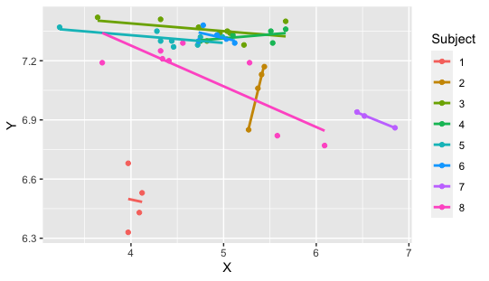 Figure 1. Recreation of “(Y) pH against (X) PaCO2 for eight subjects, with parallel lines fitted for each subject” as used in
(Bland & Altman, 1995).
Interestingly, replotting this data shows that their figure was not fully accurate (forgivable before the days of Rstudio in 1995, and not important for this example).
Figure 1. Recreation of “(Y) pH against (X) PaCO2 for eight subjects, with parallel lines fitted for each subject” as used in
(Bland & Altman, 1995).
Interestingly, replotting this data shows that their figure was not fully accurate (forgivable before the days of Rstudio in 1995, and not important for this example).
Correlation within subjects, part 2
The second part shows how to find the correlation between the subject means (Bland & Altman, 1995), number 12 on the list lit-altman_bland.md : 12. Bland JM, Altman DG. (1995) Calculating correlation coefficients with repeated observations: Part 2, correlation between subjects. 310, 633.
In this note they show the example table using the same 8 subjects with one mean observation for X and Y:
| Subject | Y | X | Number |
|---|---|---|---|
| 1 | 6.49 | 4.04 | 4 |
| 2 | 7.05 | 5.37 | 4 |
| 3 | 7.36 | 4.83 | 9 |
| 4 | 7.33 | 5.31 | 5 |
| 5 | 7.31 | 4.40 | 8 |
| 6 | 7.32 | 4.92 | 6 |
| 7 | 6.91 | 6.60 | 3 |
| 8 | 7.12 | 4.78 | 8 |
- If subject’s average Y is related to the subject’s average X
- We can use the correlation between the subject means.
They calculate the usual correlation coefficient for the mean Y and mean X; r=0.09, P=0.8. Does not take into account the different numbers of measurements on each subject.
- Does this matter?:
- Depends on how different the numbers of observations are
- whether the measurements within subjects vary much compared with the means between subjects
We can calculate a weighted correlation coefficient using the number of observations as weights. Many computer programs will calculate this, but it is not difficult to do by hand.
- They denote the mean Y and X for subject i by \(\bar{x}_i\) and \(\bar{y}_i\),
- the number of observations for subject i by \(m_i\),
- and the number of subjects by \(n\).
- The weighted mean of the \(\bar{x}_i\) is \(\frac{ \sum{ m_i \bar{x}_i } }{ \sum{ m_i } }\)
In the usual case, where there is one observation per subject, the \(m_i\) are all one and this formula gives the usual mean \(\frac{ \sum{\bar{x}_i} }{n}\).
An easy way to calculate the weighted correlation coefficient is to replace each individual observation by its subject mean. Thus the table would yield 47 pairs of observations, the first four of which would each be pH=6.49 and Paco2=4.04, and so on.
If we use the usual formula for the correlation coefficient on the expanded data we will get the weighted correlation coefficient. However, we must be careful when it comes to the P value. We have only 8 observations (n in general), not 47. We should ignore any P value printed by our computer program, and use a statistical table instead.
The formula for a weighted correlation coefficient is:
where all summations are from \(i=1\) to \(n\). When all the \(m_i\) are equal they cancel out, giving the usual formula for a correlation coefficient.
For the data in the table the weighted correlation coefficient is r=0.08, P=0.9. There is no evidence that subjects with a high Y also have a high X. However, as they have already shown in part 1, within the subject a rise in Y was associated with a fall in X.
## Code and raw data for Table I, Analysis of variance table II, and Figure 1
df <- data.frame (
  Subject = c("1", "1", "1", "1", "2", "2", "2", "2", "3", "3", "3", "3", "3", "3", "3", "3", "3", "4", "4", "4", "4", "4", "5", "5", "5", "5", "5", "5", "5", "5", "6", "6", "6", "6", "6", "6", "7", "7", "7", "8", "8", "8", "8", "8", "8", "8", "8"),

  Y = c(6.68, 6.53, 6.43, 6.33, 6.85, 7.06, 7.13, 7.17, 7.4, 7.42, 7.41, 7.37, 7.34, 7.35, 7.28, 7.3, 7.34, 7.36, 7.33, 7.29, 7.3, 7.35, 7.35, 7.3, 7.3, 7.37, 7.27, 7.28, 7.32, 7.32, 7.38, 7.3, 7.29, 7.33, 7.31, 7.33, 6.86, 6.94, 6.92, 7.19, 7.29, 7.21, 7.25, 7.2, 7.19, 6.77, 6.82),

  X = c(3.97, 4.12, 4.09, 3.97, 5.27, 5.37, 5.41, 5.44, 5.67, 3.64, 4.32, 4.73, 4.96, 5.04, 5.22, 4.82, 5.07, 5.67, 5.1, 5.53, 4.75, 5.51, 4.28, 4.44, 4.32, 3.23, 4.46, 4.72, 4.75, 4.99, 4.78, 4.73, 5.12, 4.93, 5.03, 4.93, 6.85, 6.44, 6.52, 5.28, 4.56, 4.34, 4.32, 4.41, 3.69, 6.09, 5.58)
)

# Run the Analysis of Variance with mutiple variable
name=aov(Y ~ Subject + X, data = df) #runs the ANOVA test
ls(name) #lists the items stored by the test.
summary(name) #give the basic ANOVA output.

# Output the column totals to match Altman & Bland table
df <- as.data.frame(unlist( summary(name) ))

sum(df[1:3,]) # Total Degrees of freedom
sum(df[4:6,]) # Total Sum Sq
sum(df[7:9,]) # Total Mean Sq
| Degrees of freedom | Sum of squares | Mean Square | Variance ratio (F) | Probability | |
|---|---|---|---|---|---|
| df$Subject | 7 | 2.8648 | 0.4093 | 46.60 | < 2e-16 |
| df$X | 1 | 0.1153 | 0.1153 | 13.13 | 0.000847 |
| Residuals | 38 | 0.3337 | 0.0088 |
Replicated version of Table II. Analysis of variance for the data in table I. Default R output headings modified: Degrees of freedom (Df), Sum of squares (Sum Sq), Mean square (Mean Sq), Variance ratio F (F value), Probability (Pr(>F)). (Repeated note: there is a slight varition between the published version and my replicated version of table II and Figure 1; probably due to a minor data entry error by the publisher or authors).
# code used to produce Figure 1.

require(ggplot2)
ggplot(df, aes(x = X, y = Y, group=Subject, color = Subject) ) +
  geom_point() +
  geom_smooth(aes(color = Subject), method = "lm", formula = y ~ x, , se = FALSE)

# The dataset is cited by Bland & Altman 1995 as: "Boyd O, Mackay CJ, Lamb G, Bland JM, Grounds RM, Bennett ED.Comparison of clinical information gained from routine blood-gas analysis and from gastric tonometry for intramural pH.Lancet1993;341:142–6."
References
- Bland, J. M., & Altman, D. G. (1994). Correlation, regression, and repeated data. BMJ: British Medical Journal, 308(6933), 896.
- Bland, J. M., & Altman, D. G. (1995). Statistics notes: Calculating correlation coefficients with repeated observations: Part 1—correlation within subjects. Bmj, 310(6977), 446.
- Bland, J. M., & Altman, D. G. (1995). Calculating correlation coefficients with repeated observations: Part 2—Correlation between subjects. Bmj, 310(6980), 633.
Footnote 1 This article is almost identical to the original version in acknowledgment to Altman and Bland. It is adapted here as part of a set of curated, consistent, and minimal examples of statistics required for human genomic analysis. ↩
Maintained by Dylan Lawless. Scientist at EPFL. Resume and Google scholar. RSS feed