Upervised learning K-Means clustering
- Major Requirements
- K-Means Algorithm
- Interpreting the Clusters
- Selecting the Number of Clusters
- Evaluating the Number of Clusters
- Hierarchical Clustering
This post is based on reading and figures from: Practical Statistics for Data Scientists 50+ Essential Concepts Using R and Python by Peter Bruce, Andrew Bruce, Peter Gedeck.
Clustering is a technique to divide data into different groups, where the records in each group are similar to one another. A goal of clustering is to identify significant and meaningful groups of data. The groups can be used directly, analyzed in more depth, or passed as a feature or an outcome to a predictive regression or classification model.
K-means was the first clustering method to be developed; it is still widely used, owing its popularity to the relative simplicity of the algorithm and its ability to scale to large data sets. K-means divides the data into K clusters by minimizing the sum of the squared distances of each record to the mean of its assigned cluster. This is referred to as the within-cluster sum of squares or within-cluster SS. K-means does not ensure the clusters will have the same size but finds the clusters that are the best separated.
Major Requirements
- Divide data into different groups
- Identify significant and meaningful groups of data
- Minimize the sum of the squared distances of each record to the mean of its assigned cluster
- Use within-cluster sum of squares or within-cluster SS
- Find the clusters that are the best separated
The sum of squares within a cluster is given by:
\[SS_k = \sum_{i \in Cluster_k} (x_i - x_k)^2 + (y_i - y_k)^2\]In clustering records with multiple variables (the typical case), the term cluster mean refers not to a single number but to the vector of means of the variables.
A typical use of clustering is to locate natural, separate clusters in the data. Another application is to divide the data into a predetermined number of separate groups, where clustering is used to ensure the groups are as different as possible from one another.
For example, suppose we want to divide daily stock returns into four groups. K-means clustering can be used to separate the data into the best groupings. Note that daily stock returns are reported in a fashion that is, in effect, standardized, so we do not need to normalize the data.
In R, K-means clustering can be performed using the kmeans function. For example, the following finds four clusters based on two variables—the daily stock returns for ExxonMobil (XOM) and Chevron (CVX):
df <- sp500_px[row.names(sp500_px)>='2011-01-01', c('XOM', 'CVX')]
km <- kmeans(df, centers=4)
The cluster assignment for each record is returned as the cluster component (R):
> df$cluster <- factor(km$cluster)
> head(df)
                      XOM        CVX cluster
    2011-01-03 0.73680496  0.2406809       2
    2011-01-04 0.16866845 -0.5845157       1
    2011-01-05 0.02663055  0.4469854       2
    2011-01-06 0.24855834 -0.9197513       1
    2011-01-07 0.33732892  0.1805111       2
    2011-01-10 0.00000000 -0.4641675       1
The first six records are assigned to either cluster 1 or cluster 2. The means of the clusters are also returned (R):
cluster        XOM        CVX
      1 -0.3284864 -0.5669135
      2  0.2410159  0.3342130
      3 -1.1439800 -1.7502975
      4  0.9568628  1.3708892
Clusters 1 and 3 represent “down” markets, while clusters 2 and 4 represent “up markets.”
As the K-means algorithm uses randomized starting points, the results may differ between subsequent runs and different implementations of the method. In general, you should check that the fluctuations aren’t too large.
In this example, with just two variables, it is straightforward to visualize the clusters and their means:
ggplot(data=df, aes(x=XOM, y=CVX, color=cluster, shape=cluster)) +
  geom_point(alpha=.3) +
  geom_point(data=centers,  aes(x=XOM, y=CVX), size=3, stroke=2)
The resulting plot shows the cluster assignments and the cluster means. Note that K-means will assign records to clusters, even if those clusters are not well separated (which can be useful if you need to optimally divide records into groups).
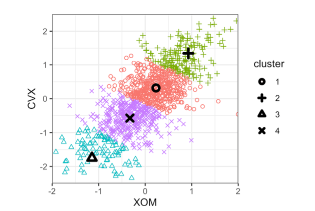
Figure 1. The clusters of K-means applied to daily stock returns for ExxonMobil and Chevron (the cluster centers are highlighted with black symbols)
K-Means Algorithm
K-means is a clustering algorithm that can be applied to a data set with p variables X1, …, Xp. While the exact solution to K-means is computationally very difficult, heuristic algorithms provide an efficient way to compute a locally optimal solution.
Major Requirements
- Specify the number of clusters K and an initial set of cluster means
- Assign each record to the nearest cluster mean as measured by squared distance
- Compute the new cluster means based on the assignment of records
- Iterate steps 2 and 3 until the assignment of records to clusters does not change
- Specify an initial set of cluster means by randomly assigning each record to one of the K clusters and then finding the means of those clusters
- Run the algorithm several times using different random samples to initialize the algorithm
- Use the iteration that has the lowest within-cluster sum of squares to get the K-means result
The sum of squares within a cluster is given by:
\[SS_k = \sum_{i \in Cluster_k} (x_i - x_k)^2 + (y_i - y_k)^2\]The nstart parameter to the R function kmeans allows you to specify the number of random starts to try. For example, the following code runs K-means to find 5 clusters using 10 different starting cluster means:
syms <- c( 'AAPL', 'MSFT', 'CSCO', 'INTC', 'CVX', 'XOM', 'SLB', 'COP',
           'JPM', 'WFC', 'USB', 'AXP', 'WMT', 'TGT', 'HD', 'COST')
df <- sp500_px[row.names(sp500_px) >= '2011-01-01', syms]
km <- kmeans(df, centers=5, nstart=10)
The function automatically returns the best solution out of the 10 different starting points. You can use the argument iter.max to set the maximum number of iterations the algorithm is allowed for each random start.
Interpreting the Clusters
An important part of cluster analysis can involve the interpretation of the clusters. The two most important outputs from kmeans are the sizes of the clusters and the cluster means.
Major Requirements
- Check the sizes of the resulting clusters with
km$size - Plot the centers of the clusters with ggplot and gather
You can plot the centers of the clusters using the gather function in conjunction with ggplot:
centers <- as.data.frame(t(centers))
names(centers) <- paste("Cluster", 1:5)
centers$Symbol <- row.names(centers)
centers <- gather(centers, 'Cluster', 'Mean', -Symbol)
centers$Color = centers$Mean > 0
ggplot(centers, aes(x=Symbol, y=Mean, fill=Color)) +
  geom_bar(stat='identity', position='identity', width=.75) +
  facet_grid(Cluster ~ ., scales='free_y')
The resulting plot reveals the nature of each cluster. For example, clusters 4 and 5 correspond to days on which the market is down and up, respectively. Clusters 2 and 3 are characterized by up-market days for consumer stocks and down-market days for energy stocks, respectively. Finally, cluster 1 captures the days in which energy stocks were up and consumer stocks were down.
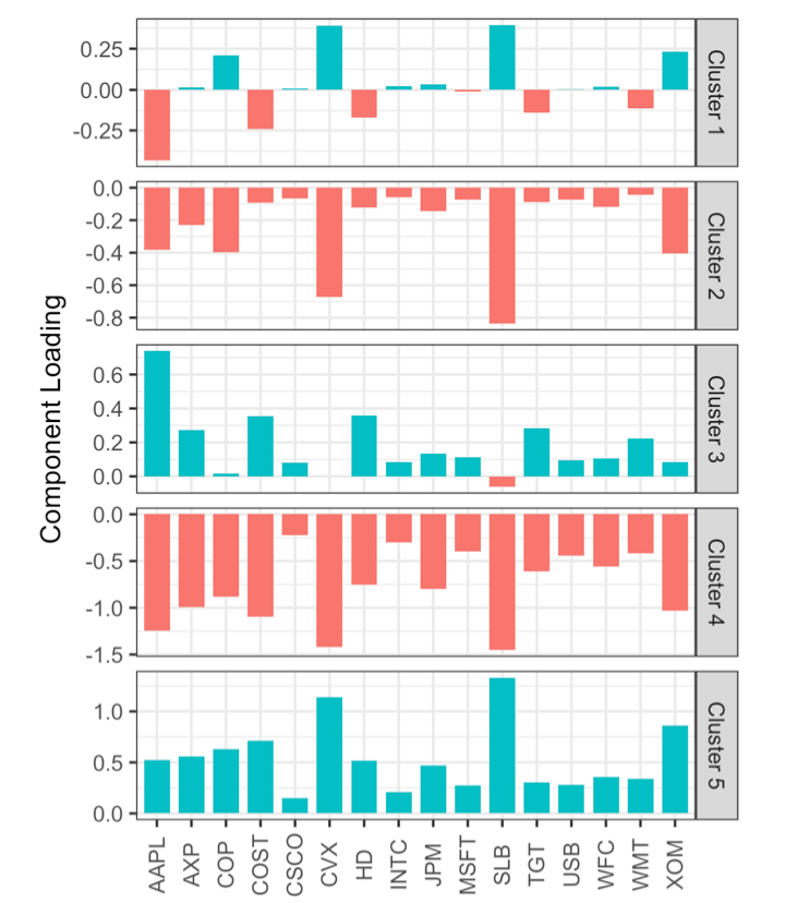
Figure 2. The means of the variables in each cluster (cluster means).
Selecting the Number of Clusters
The K-means algorithm requires that you specify the number of clusters K. Sometimes the number of clusters is driven by the application, while in other cases a statistical approach can be used.
Major Requirements
- Use practical or managerial considerations to determine the number of desired clusters
- Use a statistical approach such as the elbow method to find the “best” number of clusters
A common approach, called the elbow method, is to identify when the set of clusters explains “most” of the variance in the data. Adding new clusters beyond this set contributes relatively little in the variance explained. The elbow is the point where the cumulative variance explained flattens out after rising steeply, hence the name of the method.
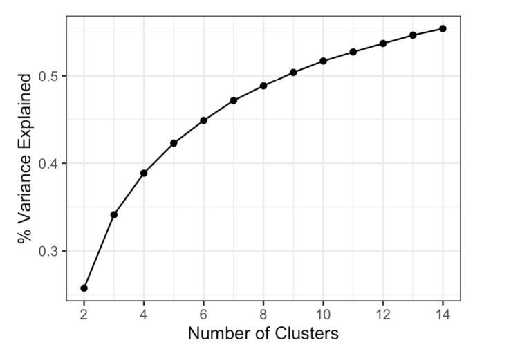
Figure 3 shows the cumulative percent of variance explained for the default data for the number of clusters ranging from 2 to 15. In this example, there is no obvious elbow point since the incremental increase in variance explained drops gradually. This is fairly typical in data that does not have well-defined clusters. This is perhaps a drawback of the elbow method, but it does reveal the nature of the data.
Evaluating the Number of Clusters
In R, the kmeans function doesn’t provide a single command for applying the elbow method, but it can be readily applied from the output of kmeans. You can evaluate how many clusters to retain by considering the replicability of the clusters on new data and whether the clusters are interpretable and related to a general characteristic of the data.
Major Requirements
- Apply the elbow method to determine the optimal number of clusters
- Use cross-validation to assess the replicability of the clusters on new data
- Consider practical considerations in choosing the number of clusters since there is no statistically determined optimal number of clusters
The algorithm iteratively assigns records to the nearest cluster mean until cluster assignments do not change, and the number of desired clusters, K, is chosen by the user.
Hierarchical Clustering
Hierarchical clustering is an alternative to K-means that can yield different clusters and is more sensitive in discovering outlying or aberrant groups or records. It allows the user to visualize the effect of specifying different numbers of clusters and lends itself to an intuitive graphical display for easier interpretation of the clusters.
Major Advantages
- Can yield different clusters than K-means
- More sensitive in discovering outlying or aberrant groups or records
- Allows visualization of the effect of specifying different numbers of clusters
- Intuitive graphical display for easier interpretation of the clusters
Hierarchical clustering involves a dendrogram that shows the relationships between clusters. The user can specify the desired number of clusters by cutting the dendrogram at a specific height.
Maintained by Dylan Lawless. Scientist at EPFL. Resume and Google scholar. RSS feed