Principal Components Analysis 1

• Introduction to PCA and SVD
• PCA: From 1-D to multi-dimensional data
• Centering the data and fitting a line
• Quantifying the fit of the line
• Principal Components (PCs)
• Variation, Eigenvalues, and Eigenvectors
• Analyzing the variation accounted for by PCs
• Visualizing PCA results
• Example R code

Introduction to PCA and SVD

• Principal Component Analysis (PCA) and Singular Value Decomposition (SVD) are powerful tools for data analysis
• Useful for visualizing and understanding high-dimensional data

PCA: From 1-D to multi-dimensional data

• Example: gene expression data with multiple variables
• PCA can help reduce dimensions and visualize data in 2-D or 3-D space
• It identifies most valuable measurements for clustering and assesses the accuracy of the reduced dimensions

Centering the data and fitting a line

• Calculate the average values of variables to find the center of the data
• Shift the plotted values to center the data on the origin (0,0)
• Fit a line through the origin that best fits the data

Quantifying the fit of the line

• PCA projects the data onto the line
• It can minimize the distance from the data to the line or maximize the distance from projected points to the origin
• Both actions are equivalent and can be described by the Pythagorean theorem:

\(a^2 = b^2 + c^2\).

Principal Components (PCs)

• Find the line that maximizes the sum of squared distances from projected points to the origin
• This line is the Principal Component 1 (PC1)
• The slope of PC1 is a linear combination of the variables (e.g., gene 1 and gene 2)
• Additional PCs can be found by following similar steps, ensuring that they are perpendicular to the previous PCs
• The number of PCs is determined by the smallest number of variables or samples

Variation, Eigenvalues, and Eigenvectors

• Calculate the variation around each PC using the sum of squared distances divided by (n-1)
• The Eigenvalue for each PC is the squared sum of distances
• The Eigenvector for each PC is the unit vector that defines the PC
• Loading scores indicate the proportions of each variable in the PC

Analyzing the variation accounted for by PCs

• Scree plot shows the percentage of variation each PC accounts for
• Can help decide how many PCs are useful for analysis
• PCs can be used as individual covariates in further analysis, such as GWAS

Visualizing PCA results

• Project data onto the most important PCs (e.g., PC1 and PC2) to create plots
• These plots can help understand the diversity within the dataset

Example R code

Here is a well-known example of PCA using the iris dataset, which is built into R. The iris dataset consists of 150 samples of iris flowers, each with four features (sepal length, sepal width, petal length, and petal width) and a species label (setosa, versicolor, or virginica).

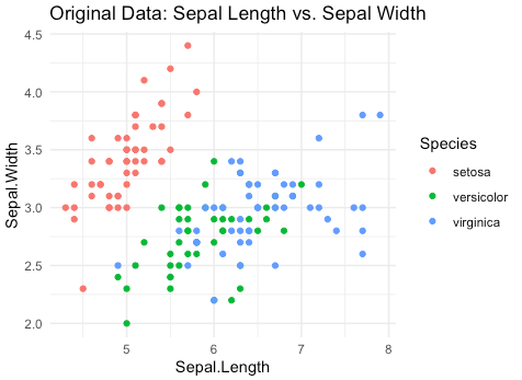
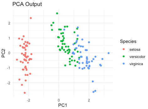
This R script first visualizes the original iris dataset, showing the relationship between sepal length and sepal width for each species. It then performs PCA on the dataset and visualizes the PCA output, which separates the three species more clearly along the first two principal components (PC1 and PC2).

# Load required libraries
library(ggplot2)
library(dplyr)

# Load the iris dataset
data(iris)

# Visualize the original data (sepal length vs. sepal width)
ggplot(iris, aes(x = Sepal.Length, y = Sepal.Width, color = Species)) +
	geom_point() +
	labs(title = "Original Data: Sepal Length vs. Sepal Width") +
	theme_minimal()

# Perform PCA
iris_pca <- prcomp(iris[, 1:4], center = TRUE, scale. = TRUE)

# Visualize the PCA output
pca_scores <- data.frame(iris_pca$x)
pca_scores$Species <- iris$Species

ggplot(pca_scores, aes(x = PC1, y = PC2, color = Species)) +
	geom_point() +
	labs(title = "PCA Output") +
	theme_minimal()