Sequence kernel association test (SKAT)
- Introduction
- Why use SKAT instead of glm?
- Kernel functions and test methods
- Examples of SKAT versus GLM
- SKAT is for joint analysis
- Interesting details
- SKAT R-package by leelabsg
- SKAT R-package: skat_logistic.R
- SKAT R-package: Kernel.R
- Related topics
- Odds ratios or betas
- Variants used in test
- Weighing variants based on deleteriousness
Introduction
The Sequence Kernel Association Test (SKAT) is a statistical method used to evaluate the association between a set of genetic variants and a phenotype, such as a disease status. This method is particularly useful for analyzing datasets containing a genotype matrix for a group of cases and controls, a phenotype file, and other covariate files. In simple terms, the SKAT method works by fitting a logistic regression model to the data, accounting for the phenotype, genotype, and other covariates. The model’s residuals and other intermediate values are then computed, and different test methods (e.g., “liu”, “liu.mod”, or “davies”) are applied based on the specific kernel function used. Finally, the method returns a list of test results, which provides insights into the association between the genetic variants and the phenotype.
Why use SKAT instead of glm?
The glm (Generalized Linear Model) function in R is a more general statistical tool used to fit various types of linear models, such as logistic regression, Poisson regression, and others, depending on the chosen distribution family. The glm function can be applied to a wide range of problems, not just limited to genetic data analysis.
In contrast, the Sequence Kernel Association Test (SKAT) method is specifically designed for genetic data analysis and aims to assess the joint effect of multiple genetic variants on a phenotype. While SKAT does utilize logistic regression (which can be performed using the glm function) as a part of its process, it goes beyond just fitting a single model. SKAT incorporates kernel functions and different test methods to evaluate the association between sets of genetic variants and phenotypes.
In summary, the key difference between using the R glm function and the SKAT method is their scope and purpose. The glm function is a general-purpose tool for fitting linear models, while the SKAT method is a specialized approach for analyzing the association between genetic variants and phenotypes by leveraging kernel functions and test methods in addition to logistic regression.
Kernel functions and test methods
kernel functions and different test methods are essential components of the Sequence Kernel Association Test (SKAT) method, as they help to capture and quantify the association between sets of genetic variants and phenotypes.
Kernel Functions:
A kernel function is a mathematical function that measures the similarity or association between two data points in a high-dimensional space. In the context of SKAT, kernel functions are used to compute the association between genetic variants, considering their joint effects on the phenotype. Some commonly used kernel functions in SKAT are:
- Linear kernel: This kernel measures the linear relationship between genetic variants. It is the simplest form and is calculated as the dot product of the input data points.
- Linear weighted kernel: Similar to the linear kernel, but it incorporates weights, allowing for the adjustment of the importance of each genetic variant in the analysis.
- Other kernels: Depending on the study, researchers can also use other kernel functions, such as the polynomial, Gaussian (RBF), or exponential kernels, which might better capture the underlying relationships in the data.
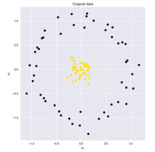
There is a brilliant explanation here: https://stats.stackexchange.com/questions/152897/how-to-intuitively-explain-what-a-kernel-is
If we could find a higher dimensional space in which these points were linearly separable, then we could do the following:
- Map the original features to the higher, transformer space (feature mapping)
- Perform linear SVM in this higher space
- Obtain a set of weights corresponding to the decision boundary hyperplane
- Map this hyperplane back into the original 2D space to obtain a non linear decision boundary
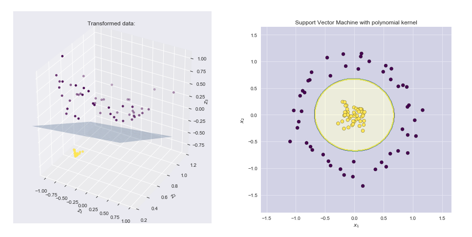
Visualizing the feature map and the resulting boundary line
- Left-hand side plot shows the points plotted in the transformed space together with the SVM linear boundary hyperplane
- Right-hand side plot shows the result in the original 2-D space
Test Methods:
Test methods in SKAT are statistical approaches used to compute the p-values for the association between the sets of genetic variants and the phenotype. These p-values indicate the significance of the association. Some common test methods used in SKAT are:
- Liu method: This method uses a moment-matching technique to approximate the null distribution of the test statistic. It is computationally efficient and provides accurate p-values for most scenarios.
- Liu modified method (liu.mod): A modified version of the Liu method, which improves the accuracy of the p-value estimation in certain cases.
- Davies method: This method computes the p-value using the characteristic function of the null distribution of the test statistic. While it can be more accurate than the Liu method, it is computationally more intensive and might not be suitable for large-scale datasets.
In summary, kernel functions and test methods are integral parts of the SKAT method, helping to model the complex relationships between genetic variants and phenotypes and providing statistical significance measures for the associations.
Examples of SKAT versus GLM
NOTE: simplified code which will not run as-is.
In this example, we will compare the use of the SKAT method with the glm function for a dataset consisting of a genotype matrix, phenotype file, and other covariates. For simplicity, we will assume that the dataset has already been loaded and processed into the appropriate format.
Using glm function:
First, we will fit a logistic regression model for each genetic variant in the genotype matrix, adjusting for covariates, and compute a p-value for each variant.
# Load the required libraries
library(glm)

# Assume 'genotype_matrix', 'phenotype', and 'covariates' are already loaded and pre-processed

# Initialize a vector to store p-values for each genetic variant
p_values <- numeric(ncol(genotype_matrix))

# Fit a logistic regression model for each genetic variant and compute p-values
for (i in 1:ncol(genotype_matrix)) {
  model <- glm(phenotype ~ genotype_matrix[, i] + covariates, family = "binomial")
  p_values[i] <- summary(model)$coefficients[2, 4]
}

# Now 'p_values' contains the p-values for each genetic variant
Using SKAT:
Next, we will use the SKAT method to assess the joint effect of multiple genetic variants on the phenotype, adjusting for covariates.
# Load the required libraries
library(SKAT)

# Assume 'genotype_matrix', 'phenotype', and 'covariates' are already loaded and pre-processed

# Fit a SKAT logistic model for the genotype matrix, adjusting for covariates
skat_result <- SKAT_Logistic(Z = genotype_matrix,
                             y = phenotype,
                             X1 = covariates,
                             kernel = "linear",
                             method = "liu")

# Extract the p-value for the association between genetic variants and phenotype
skat_p_value <- skat_result$p.value
In this example, the glm approach computes a p-value for each genetic variant individually, without considering their joint effects on the phenotype. On the other hand, the SKAT method evaluates the association between a set of genetic variants and the phenotype, taking into account their joint effects, which may provide more insights into the complex relationships between genetic variants and phenotypes.
SKAT is for joint analysis
SKAT does not analyze each variant independently and report a p-value for each variant like a single-variant analysis approach would. Instead, SKAT evaluates the joint effects of multiple genetic variants on the phenotype and reports a single p-value for the association between the set of genetic variants and the phenotype.
SKAT is designed to detect the cumulative effects of multiple rare and common variants within a gene or a genomic region, which could be missed in single-variant analyses due to the low frequency or small effect size of individual variants. By testing the joint effects of multiple variants, SKAT can potentially identify associations that would be difficult to detect in a single-variant analysis.
If you group variants by genes, SKAT will perform a joint analysis of all variants within each gene and report a gene-level p-value. This approach allows you to assess the combined effects of multiple genetic variants within a gene on the phenotype, which can be particularly helpful for identifying associations driven by rare and common variants with small individual effects that may not be detected in single-variant analyses.
Adding a gene term to the glm model is not equivalent to a gene-level SKAT analysis. When you include a gene term in a glm model, you are assuming that all variants within the same gene have the same effect on the phenotype, which might not be the case, especially when considering complex traits or diseases.
SKAT, on the other hand, takes into account the joint effects of multiple genetic variants within a gene on the phenotype, without assuming that all variants have the same effect. It assesses the association between a set of genetic variants and the phenotype by considering different weights for each variant (based on the kernel function) and their combined effects.
Thus, while a glm model with a gene term can provide an overall assessment of the association between a gene and the phenotype, it does not account for the individual effects and potential interactions between variants within the gene. In contrast, SKAT’s gene-level analysis can provide a more comprehensive understanding of the combined effects of genetic variants within a gene on the phenotype.
Interesting details
We have covered the major concepts and applications of SKAT, but a statistics expert may be interested in considering the following additional technical details:
- Choice of kernel function: The choice of kernel function can influence the results of SKAT. While the linear kernel is the default choice and widely used, other kernel functions like the “linear.weighted” kernel, which assigns weights to variants based on their minor allele frequency, can be more powerful in certain scenarios. Selecting an appropriate kernel function depends on the specific study and the underlying genetic architecture.
- Rare variant analysis: SKAT is particularly useful for rare variant analysis, where traditional single-variant methods often lack power due to the low frequency of rare variants. By aggregating the effects of multiple rare variants within a gene or genomic region, SKAT can detect associations that may be missed by single-variant approaches.
- Adjusting for population stratification: Like other genetic association tests, SKAT results can be confounded by population stratification. It is important to consider and adjust for potential population stratification by including principal components or other relevant covariates in the analysis to control for the confounding effects.
- Multiple testing correction: When performing SKAT on multiple genes or genomic regions, it is essential to correct for multiple testing to control the false positive rate. Methods like Bonferroni correction, false discovery rate (FDR) control, or family-wise error rate (FWER) control can be used to account for multiple testing and adjust the p-values accordingly.
- Gene-gene interactions and other extensions: While the standard implementation of SKAT tests for the joint effects of genetic variants within a single gene or genomic region, researchers may also be interested in exploring gene-gene interactions or more complex relationships between genetic variants and phenotypes.
- Extensions of SKAT, like SKAT-O (Optimal) or other multivariate methods, can be used to analyze more complex models and relationships in genetic data. These technical details can be relevant for a statistics expert when designing, conducting, and interpreting the results of SKAT analyses in genetic studies.
SKAT R-package by leelabsg
The following discussions are code are based on the github repo
- https://github.com/leelabsg/SKAT While all the functions in the SKAT package have specific roles in various aspects of the analysis, here are some of the key functions that may be particularly important to note for the usage of SKAT:
-
MAIN.R: This file contains the main SKAT function for continuous phenotypes, SKAT(). It is the primary function for conducting SKAT on continuous outcomes. -
SKAT_Logistic.R: We will discuss this in detail. This file contains the main function for binary phenotypes, SKAT.logistic(). It is the primary function for conducting SKAT on binary outcomes, such as case-control studies. -
SKAT_Optimal.R: This file contains the implementation of the SKAT-O (Optimal) method, which is an extension of SKAT that adaptively combines the burden test and SKAT to achieve optimal power across a wider range of scenarios. -
Null_Model.R: This file contains the functions to fit the null model that is used as a reference in the association test. It is important because it provides the baseline model for the association tests and helps control for potential confounders. -
SSD.R: This file contains functions related to the SSD (Sequence Kernel Association Test Set-based Single variant Data) format, which is a compact file format designed to store genotype and phenotype data for SKAT analyses. It is useful for handling large-scale genetic data efficiently. -
Kernel.R: We will discuss this in detail. This file contains functions to compute different kernel matrices for SKAT. The choice of kernel function can impact the test’s performance, and understanding the available kernel functions can help in selecting the appropriate one for a specific analysis.
These functions are essential for various aspects of SKAT analysis, and users should be familiar with them to effectively use the SKAT package. However, depending on the specific needs of a study, other functions in the package might also be relevant.
Main Functions and key references
Following are main functions and key references. For details, please refer the package manual and vignettes.
- SKAT function: Burden test, SKAT, and SKAT-O
- Lee, S., Emond, M.J., …, and Lin, X. (2012). Optimal unified approach for rare variant association testing with application to small sample case-control whole-exome sequencing studies. AJHG, 91, 224-237.
- Lee, S., Wu, M. and Lin, X. (2012). Optimal tests for rare variant effects in sequencing association studies. Biostatistics, 13, 762-775
- Wu, M., Lee, S., Cai, T., Li, Y., Boehnke, M. and Lin, X. (2011). Rare Variant Association Testing for Sequencing Data Using the Sequence Kernel Association Test (SKAT). AJHG, 89, 82-93.
- Robust approaches functions for binary traits: SKATBinary_Robust and SKAT_CommonRare_Robust
- Zhao, Z., Bi, W., Zhou, W., VanderHaar, P., Fritsche, L.G., Lee, S. (2020) UK Biobank Whole-Exome Sequence Binary Phenome Analysis with Robust Region-based Rare-Variant Test. AJHG, 2020, 3-12.
- SKATBinary function: Burden test, SKAT, and SKAT-O with efficient resampling for binary traits
- Lee, S., Fuchsberger, C., Kim, S., Scott, L. (2016) An efficient resampling method for calibrating single and gene-based rare variant association analysis in case-control studies, Biostatistics, 17, 1-15.
- SKAT_CommonRare function: joint test for common and rare variants
- Ionita-Laza, I., Lee, S., Makarov, V., Buxbaum, J. Lin, X. (2013). Sequence kernel association tests for the combined effect of rare and common variants. AJHG, 92, 841-853.
- SKAT_ChrX function: X-chromosome test
- Ma, C., Boehnke, M., Lee, S. and the GoT2D investigators (2015) Evaluating the calibration and power of three gene-based association tests for the X chromosome, Genetic Epidemiology, 39, 499-508.
- SKAT_NULL_emmaX function: Kinship adjustment
- SSD functions: plink binary file related functions
- Power_Continuous, …: power calculation functions
Link
- SKAT CRAN: Link
- SKAT google group: Link
- Example dataset: Link
The following description is based on one of the main SKAT functions -SKAT_Logistic.Rwhich is most likely to be used.
SKAT R-package: skat_logistic.R
The following discussions are code are based on the github repo
Simplified description
- Function definition:
SKAT.logistic.Linear:- Takes input parameters and calls appropriate functions based on conditions
- Function definition:
KMTest.logistic.Linear:- Processes input based on kernel, weights, and correlation parameter
- Computes test statistic
Q - Computes resampling test statistic if required
- Computes weight matrix
- Calls the appropriate test method
- Returns test results in a list
- Function definition:
SKAT.logistic.Other:- Computes kernel matrix if not provided
- Computes test statistic
Q - Computes resampling test statistic if required
- Computes weight matrix based on the method
- Calls the appropriate test method
- Returns test results in a list
- Main function definition:
SKAT.logistic:- Fits a logistic regression model using
glm - Computes residuals, probabilities, and other intermediate values
- Calls appropriate functions based on conditions
- Returns test results in a list
- Fits a logistic regression model using
Description with full variables
- Function definition:
SKAT.logistic.Linear. The function takes the following input parameters:-
res: Residuals -
Z: Genotype matrix -
X1: Covariate matrix -
kernel: Kernel function -
weights: Optional weights for kernel -
pi_1: Vector of probabilities -
method: Test method, e.g., “liu”, “liu.mod”, “davies” -
res.out: Residuals for resampling -
n.Resampling: Number of resampling iterations -
r.corr: Correlation parameter -
IsMeta: Boolean flag for MetaSKAT
-
- Check the conditions and call appropriate functions:
- If
IsMetais TRUE, call theSKAT_RunFrom_MetaSKATfunction - If the length of
r.corris 1, call theKMTest.logistic.Linear function - Otherwise, call the
SKAT_Optimal_Logisticfunction
- If
- Function definition:
KMTest.logistic.Linear:- Similar input parameters as
SKAT.logistic.Linear - Process the input based on the provided kernel, weights, and correlation parameter
- Compute the test statistic
Q - Compute the resampling test statistic
Q.resifn.Resamplingis greater than 0 - Compute the weight matrix
W.1 - Call the appropriate test method: “liu”, “liu.mod”, or “davies”
- Return the test results in a list
- Similar input parameters as
- Function definition:
SKAT.logistic.Other:- Similar input parameters as
SKAT.logistic.Linear - Compute the kernel matrix
Kif not provided - Compute the test statistic
Q - Compute the resampling test statistic
Q.resifn.Resamplingis greater than 0 - Compute the weight matrix
Wbased on the method - Call the appropriate test method: “liu”, “liu.mod”, or “davies”
- Return the test results in a list
- Similar input parameters as
- Main function definition:
SKAT.logistic:- The function takes the following input parameters:
-
Z: Genotype matrix -
y: Phenotype vector -
X1: Covariate matrix -
kernel: Kernel function -
weights: Optional weights for kernel -
method: Test method, e.g., “liu”, “liu.mod”, “davies” -
res.out: Residuals for resampling -
n.Resampling: Number of resampling iterations -
r.corr: Correlation parameter
-
- Fit a logistic regression model using the
glmfunction - Compute residuals, probabilities, and other intermediate values
- If method is “var.match”, call the
KMTest.logistic.Linear.VarMatchingfunction - If the kernel is “linear” or “linear.weighted” and the number of samples is greater than the number of variables, call the
SKAT.logistic.Linearfunction - Otherwise, call the
SKAT.logistic.Otherfunction - Return the test results in a list
- The function takes the following input parameters:
Original code: skat_logistic.R
SKAT.logistic.Linear = function(res,Z,X1, kernel, weights = NULL, pi_1, method,res.out,n.Resampling,r.corr, IsMeta=FALSE){


	if(length(r.corr) > 1 && dim(Z)[2] == 1){
		r.corr=0
	}

	if(IsMeta){

		re = SKAT_RunFrom_MetaSKAT(res=res,Z=Z, X1=X1, kernel=kernel, weights=weights, pi_1=pi_1
		, out_type="D", method=method, res.out=res.out, n.Resampling=n.Resampling, r.corr=r.corr)

	} else if(length(r.corr) == 1 ){

		re = KMTest.logistic.Linear(res,Z,X1, kernel, weights, pi_1, method
		, res.out, n.Resampling, r.corr)

	} else {


		re =SKAT_Optimal_Logistic(res, Z, X1, kernel, weights, pi_1, method
		, res.out, n.Resampling, r.corr)

	}

	return(re)
}

#
#	Modified by Seunggeun Lee - Ver 0.1
#

KMTest.logistic.Linear = function(res, Z, X1, kernel, weights = NULL, pi_1, method,res.out,n.Resampling,r.corr){

  # Weighted Linear Kernel
  if (kernel == "linear.weighted") {
    Z = t(t(Z) * (weights))
  }

  # r.corr
  if(r.corr == 1){
  	Z<-cbind(rowSums(Z))
  } else if(r.corr > 0){

   	p.m<-dim(Z)[2]
	R.M<-diag(rep(1-r.corr,p.m)) + matrix(rep(r.corr,p.m*p.m),ncol=p.m)
	L<-chol(R.M,pivot=TRUE)
	Z<- Z %*% t(L)
  }

  # Get temp
  Q.Temp = t(res)%*%Z
  Q = Q.Temp %*% t(Q.Temp)/2

  Q.res = NULL
  if(n.Resampling > 0){
  	Q.Temp.res = t(res.out)%*%Z
  	Q.res = rowSums(rbind(Q.Temp.res^2))/2
  }

  #gg = X1%*%solve(t(X1)%*%(X1 * pi_1))%*%t(X1 * pi_1)  ### Just a holder... not all that useful by itself
  #P0 = D-(gg * pi_1)      ### This is the P0 or P in Zhang and Lin
  # P0 = D-D%*%gg
  # P0 = D- D%*%X1%*%solve(t(X1)%*%(X1 * pi_1))%*%t(X1) %*% D

  #W = P0%*%K
  #W = K * pi_1 - (X1 *pi_1) %*%solve(t(X1)%*%(X1 * pi_1))%*% ( t(X1 * pi_1) %*% K)
  #muq  = sum(diag(W))/2   # this is the same as e-tilde

  # tr(W W) = tr(P0 K P0 K ) = tr ( Z^T P0 Z Z^T P0 Z ) = tr( P0 Z Z^T P0 Z Z^T )
  # tr(P0 K P0)
  # tr(A B) = tr(A * t(B))

  W.1 = t(Z) %*% (Z * pi_1) - (t(Z * pi_1) %*%X1)%*%solve(t(X1)%*%(X1 * pi_1))%*% (t(X1) %*% (Z * pi_1)) # t(Z) P0 Z


  if( method == "liu" ){
	out<-Get_Liu_PVal(Q, W.1, Q.res)
  } else if( method == "liu.mod" ){
	out<-Get_Liu_PVal.MOD(Q, W.1, Q.res)
  } else if( method == "davies" ){
	out<-Get_Davies_PVal(Q, W.1, Q.res)
  } else {
	stop("Invalid Method!")
  }


  re<-list(p.value = out$p.value, p.value.resampling = out$p.value.resampling, Test.Type = method, Q = Q,  Q.resampling = Q.res, param=out$param )
  return(re)
}


SKAT.logistic.Other = function(res, Z, X1, kernel , weights = NULL, pi_1, method,res.out,n.Resampling){

  n = nrow(Z)
  m = ncol(Z)

  # If m >> p and ( linear or linear.weight) kernel than call
  # Linear function

  if (Check_Class(kernel, "matrix")) {
    K = kernel
  } else {
    K = lskmTest.GetKernel(Z, kernel, weights,n,m)
  }


  Q = t(res)%*%K%*%res/2
  Q.res = NULL
  if(n.Resampling > 0){
	Q.res<-rep(0,n.Resampling)
	for(i in 1:n.Resampling){
  		Q.res[i] = t(res.out[,i])%*%K%*%res.out[,i]/2
  	}
  }

  D  = diag(pi_1)
  gg = X1%*%solve(t(X1)%*%(X1 * pi_1))%*%t(X1 * pi_1)  ### Just a holder... not all that useful by itself
  P0 = D-(gg * pi_1)      ### This is the P0 or P in Zhang and Lin
  # P0 = D-D%*%gg

  if(method == "davies"){
  	P0_half = Get_Matrix_Square.1(P0)
	#print(dim(P0_half))
	W1 = P0_half %*% K %*% t(P0_half)
  } else {
	#W    = P0%*%K
  	W = K * pi_1 - (X1 *pi_1) %*%solve(t(X1)%*%(X1 * pi_1))%*% ( t(X1 * pi_1) %*% K)
  }

  if( method == "liu" ){
	out<-Get_Liu_PVal(Q, W, Q.res)
  } else if( method == "liu.mod" ){
	out<-Get_Liu_PVal.MOD(Q, W, Q.res)
  } else if( method == "davies" ){
	out<-Get_Davies_PVal(Q, W1, Q.res)
  } else {
	stop("Invalid Method!")
  }

  re<-list(p.value = out$p.value, p.value.resampling = out$p.value.resampling, Test.Type = method, Q = Q, param=out$param )
  return(re)

}

#
#	Modified by Seunggeun Lee - Ver 0.3
# 	method : satterth, liu

SKAT.logistic = function(Z,y,X1, kernel = "linear", weights = NULL, method="liu"
, res.out=NULL, n.Resampling = 0, r.corr=r.corr){


	n = length(y)
	m = ncol(Z)

	glmfit= glm(y~X1 -1, family = "binomial")
 	betas = glmfit$coef
  	mu    = glmfit$fitted.values
  	eta   = glmfit$linear.predictors

	mu    = glmfit$fitted.values
	pi_1 = mu*(1-mu)
  	res = y- exp(eta)/(1+exp(eta))

	if(method=="var.match"){
		re = KMTest.logistic.Linear.VarMatching(res, Z, X1, kernel, weights, pi_1, method,res.out,n.Resampling,r.corr, mu)
		return(re)
	}

	# If m >> p and ( linear or linear.weight) kernel than call
	# Linear function
	if( (kernel =="linear" || kernel == "linear.weighted") && n > m){
		re = SKAT.logistic.Linear(res,Z,X1, kernel, weights , pi_1,method,res.out,n.Resampling,r.corr=r.corr)
	} else {
		re = SKAT.logistic.Other(res,Z,X1, kernel, weights, pi_1, method,res.out,n.Resampling)
	}

	return(re)
}
SKAT R-package: Kernel.R
The following discussions are code are based on the github repo
Simplified description: Kernal.R
- Define helper function
K1_Helpfor 2-way interaction kernel - Define function
call_Kernel_IBSto calculate Identity-By-State (IBS) kernel - Define function
call_Kernel_IBS_Weightto calculate weighted IBS kernel - Define function
call_Kernel_2wayIXto calculate 2-way interaction kernel - Define main function
lskmTest.GetKernelto calculate kernel matrix based on specified kernel type:- If kernel is “quadratic”, compute quadratic kernel matrix
- If kernel is “IBS”, compute IBS kernel matrix using
call_Kernel_IBS - If kernel is “IBS.weighted”, compute weighted IBS kernel matrix using
call_Kernel_IBS_Weight - If kernel is “2wayIX”, compute 2-way interaction kernel matrix using
call_Kernel_2wayIX - If kernel is “IBS.weighted_OLD”, compute weighted IBS kernel matrix using an older method
- If kernel is “IBS_OLD”, compute IBS kernel matrix using an older method
- If kernel is “2wayIX_OLD”, compute 2-way interaction kernel matrix using an older method
- Return the computed kernel matrix
Original code: Kernel.R
K1_Help= function(x,y){
  # Helper function for 2 way interaction kernel
  p = length(x)
  a = x*y
  b = cumsum(a)
  return(sum(a[-1]*b[-p]))
}

call_Kernel_IBS<-function(Z,n,p){

	#Kernel_IBS(double * Z, int * pn, int * pp, double * Kernel)
	K<- matrix(rep(0,n*n),nrow = n, ncol = n)
	temp<-.C("Kernel_IBS",as.integer(as.vector(t(Z))),as.integer(n), as.integer(p),as.double(as.vector(K)))[[4]]
	matrix(temp,nrow=n)
}

call_Kernel_IBS_Weight<-function(Z,n,p,weights){

	#Kernel_IBS_Weight(int * Z, int * pn, int * pp, int *UseGivenWeight ,  double * weight, double * Kernel)
	given_weight = 1;
	if( is.null(weights)){
		weights = rep(0,p);
		given_weight = 0;
	} else {
		# change!!
		weights<-weights^2;
	}
	K<- matrix(rep(0,n*n),nrow = n, ncol = n)
	temp<-.C("Kernel_IBS_Weight",as.integer(as.vector(t(Z))),as.integer(n), as.integer(p),as.integer(given_weight),
	as.double(weights),as.double(as.vector(K)))[[6]]
	matrix(temp,nrow=n)
}

call_Kernel_2wayIX<-function(Z,n,p){

	#Kernel_IBS(double * Z, int * pn, int * pp, double * Kernel)
	K<- matrix(rep(0,n*n),nrow = n, ncol = n)
	temp<-.C("Kernel_2wayIX",as.integer(as.vector(t(Z))),as.integer(n), as.integer(p),as.double(as.vector(K)))[[4]]
	matrix(temp,nrow=n)
}

lskmTest.GetKernel = function(Z, kernel, weights,n,m){

    	if (kernel == "quadratic") {
      		K = (Z%*%t(Z)+1)**2
    	}


	if (kernel == "IBS") {
      		K = call_Kernel_IBS(Z,n,m)
    	}
    	if (kernel == "IBS.weighted") {

      		K = call_Kernel_IBS_Weight(Z,n,m,weights)
    	}
  	if (kernel == "2wayIX") {
      		K = call_Kernel_2wayIX(Z,n,m)
    	}
   	if (kernel == "IBS.weighted_OLD") {
      		#K = matrix(nrow = n, ncol = n)
      		if (is.null(weights)) {
        		qs = apply(Z, 2, mean)/(2)
        		weights = 1/sqrt(qs)
      		} else {
			weights<-weights^2
		}
      		K1 = matrix(nrow =n, ncol = n)
      		for (i in 1:n) {
        		K1[i,] = apply(abs(t(Z)-Z[i,])*weights,2, sum)
      		}
      		K= 1-(K1)/(2*sum(weights))
    	}

    	if (kernel == "IBS_OLD") {
      		K1=matrix(nrow=n,ncol=n)
      		for (i in 1:n) {
        		K1[i,] = apply(abs(t(Z)-Z[i,]),2, sum)
      		}
      		K = (2*m-K1)/(2*m)
    	}
   	if (kernel == "2wayIX_OLD") {
      		K = 1+Z%*%t(Z)
      		N1=  matrix(nrow = n, ncol = n)
      		for (i in 1:n){
        		for (j in i:n){
	    			N1[j,i] = N1[i,j] = K1_Help(Z[i,], Z[j,])
	  		}
      		}
      		K = K+N1
    	}
	return(K)

}

#.First.lib <- function(lib, pkg) { library.dynam('SKAT', pkg, lib) }
Related topics
Other statistics topics
The methods used in SKAT have their roots in more general statistical protocols. The foundation of SKAT lies in kernel machine regression, which is a versatile and powerful statistical method that can be applied to various fields outside genetics. Kernel methods are a class of algorithms for pattern analysis and are particularly useful for capturing complex, non-linear relationships in data.
Some of the background concepts that contribute to the development of kernel methods and, by extension, SKAT, include:
- Regression analysis: A fundamental concept in statistics, regression analysis is used to model and analyze relationships between variables. Linear regression is a simple, widely-used form of regression analysis that models the relationship between a dependent variable and one or more independent variables.
- Generalized linear models (GLMs): GLMs are a class of flexible regression models that extend linear regression by allowing the dependent variable to follow a distribution other than the normal distribution. This flexibility makes GLMs particularly useful for analyzing different types of data, including binary, count, and continuous data.
- Kernel functions: Kernel functions play a crucial role in kernel methods. They are used to map data from an original lower-dimensional space to a higher-dimensional space, which often reveals complex relationships that are not apparent in the original space. Common kernel functions include the linear, polynomial, radial basis function (RBF), and sigmoid kernels.
- Support Vector Machines (SVMs): SVMs are a class of supervised learning models that have been widely applied in classification and regression tasks. They use kernel functions to transform input data into a higher-dimensional space and find the optimal decision boundary (hyperplane) to separate different classes or predict the target variable.
- Regularization techniques: Regularization techniques, such as ridge regression and LASSO, are used to prevent overfitting in regression models by adding a penalty term to the model’s loss function. Regularization helps to constrain the model complexity and make it more generalizable to unseen data.
These general statistical concepts, along with the specific needs and challenges of genetic association studies, have shaped the development of the Sequence Kernel Association Test (SKAT) and made it a powerful and flexible tool for analyzing rare variant associations in genetic data.
Other fundamental topics
There are several fundamental statistical and mathematical concepts that underlie the development of kernel methods and their applications, including SKAT. Some of these foundational concepts include:
Probability theory: Probability theory is a branch of mathematics that deals with the analysis of random phenomena. It provides the basis for understanding and modeling uncertainty in data and is a fundamental concept in statistical analysis. Bayesian statistics: Bayesian statistics is an approach to statistical inference that incorporates prior knowledge about the parameters of interest. It relies on Bayes’ theorem to update the probabilities of different hypotheses as new data is observed. Bayesian methods have been influential in the development of many machine learning algorithms, including kernel methods. Linear algebra: Linear algebra deals with vector spaces and linear mappings between them. It provides the foundation for understanding and manipulating high-dimensional data, which is often required in kernel methods. Optimization: Optimization is the process of finding the best solution to a problem, often by minimizing or maximizing a particular function. Many machine learning algorithms, including kernel methods, rely on optimization techniques to find the best model parameters given the observed data. Matrix factorization and decomposition: Techniques such as singular value decomposition (SVD) and eigenvalue decomposition play a crucial role in dimensionality reduction, a common preprocessing step in machine learning and data analysis. These techniques help to reveal the underlying structure in data and can improve the performance of kernel methods. Functional analysis: Functional analysis is a branch of mathematics that deals with the study of spaces of functions and the operators acting upon them. It provides the theoretical basis for understanding the behavior of kernel functions and their properties, which is critical for the development and application of kernel methods. These foundational concepts have shaped the development of kernel methods and their applications in various fields, including genetics, where they have been adapted and extended to address specific challenges in the analysis of rare variant associations.
Other Bayesian topics
Bayesian statistics has interesting opportunities - but note SKAT itself is not directly based on this. Instead, it is a frequentist method that uses kernel machine regression models to perform gene-based tests for the association between genetic variants and a phenotype of interest. The method relies on combining variant-level information by constructing a kernel matrix representing the similarity between individuals and then using a variance component score test to evaluate the association.
Bayesian statistics was mentioned as part of the general background for kernel methods, but it is not a direct component of SKAT. However, Bayesian statistical methods have been applied to other gene-based tests and genetic association studies. These methods can incorporate prior knowledge and model complex structures in the data, but they are not specifically used in the context of SKAT.
it is possible to develop a Bayesian counterpart to the SKAT method. While SKAT itself is based on frequentist statistics, the underlying idea of aggregating variant-level information and testing the association between genetic variants and a phenotype can be adapted to a Bayesian framework.
To do so, you would need to:
- Define a Bayesian hierarchical model for the genetic data, which includes specifying prior distributions for the model parameters (e.g., effect sizes, variance components).
- Develop a method to aggregate the variant-level information within genes or genomic regions, which could involve designing a suitable kernel function or another way to combine variant effects.
- Use Bayesian inference techniques (such as Markov Chain Monte Carlo or Variational Inference) to estimate the posterior distributions of the model parameters, given the observed data.
- Compute posterior probabilities or Bayes factors to assess the strength of the association between the genetic variants and the phenotype of interest.
While this would be a different method than SKAT, it would share the same goal of conducting gene-based tests for genetic association studies. Keep in mind that developing and implementing a Bayesian version of SKAT would be a non-trivial task and could involve additional computational challenges. However, it could potentially offer benefits such as incorporating prior knowledge and providing more interpretable measures of evidence for the associations.
Other joint analysis topics
There are several methods for joint analysis of genetic variants in genomics besides SKAT. Each method has its own strengths and weaknesses, and their performances may vary depending on the specific genetic architecture of the traits being studied. Some popular methods include:
- Burden tests: These methods collapse variants within a gene or genomic region into a single genetic score and then test for an association between the score and the phenotype. Examples of burden tests include the Cohort Allelic Sums Test (CAST), the Combined Multivariate and Collapsing (CMC) method, and the Variable Threshold (VT) method.
- Sequence kernel association test (SKAT-O): SKAT-O is an extension of the SKAT method that combines both burden and dispersion components to improve power across different scenarios. It provides a unified test that adaptively weighs the contributions of rare and common variants, making it more robust to various genetic architectures.
- Adaptive Sum of Powered Score (aSPU) test: aSPU is a flexible gene-based test that uses an adaptive combination of score tests with different weights for rare and common variants. This method allows for improved power across a wide range of genetic architectures.
- Rare variant generalized linear mixed model (rvGLMM): This method is based on generalized linear mixed models and is designed to handle rare variant data. It can accommodate various types of phenotypes and allows for both gene-based and variant-based association tests.
- Bayesian methods: Bayesian methods like the Bayesian variable selection regression (BVSR) or Bayesian group lasso can be used for joint analysis of genetic variants. These methods incorporate prior knowledge and allow for simultaneous estimation of the effect sizes of multiple genetic variants while accounting for complex genetic architectures.
The choice of the method depends on the specific research question, the genetic architecture of the trait, and the type of genomic data being analyzed. Comparing the performance of different methods using simulation studies or cross-validation can help identify the most suitable approach for a given study.
Odds ratios or betas
NOTE: code not tested - still in work.
A on the user forum, someone asks if it is possible to obtain odds ratios or betas. https://groups.google.com/g/skat_slee/c/9BklI9n-H1w While it’s not possible directly from the SKAT package, you can still estimate them under the burden test framework using a genotype matrix.
The Burden test framework collapses the genotype matrix for each gene into a single genetic score. To calculate the betas or odds ratios for each gene, you can follow these steps:
- Collapse the genotype matrix into a genetic score for each gene.
- Use logistic regression (for case-control data) or linear regression (for quantitative trait data) to model the phenotype using the genetic score and covariates.
- Obtain the betas (for linear regression) or odds ratios (for logistic regression) from the regression model.
Here’s an example of how you could calculate the betas for the burden test using R:
# Assuming you have a genotype matrix `G`, a phenotype vector `Y`, and a covariate matrix `C`

# Collapse the genotype matrix for each gene into a single genetic score
genetic_score <- rowSums(G)

# Perform linear regression
linear_model <- lm(Y ~ genetic_score + C)

# Obtain the betas for each gene
beta <- coef(linear_model)["genetic_score"]
And for calculating the odds ratios for case-control data:
# Assuming you have a genotype matrix `G`, a binary phenotype vector `Y`, and a covariate matrix `C`

# Collapse the genotype matrix for each gene into a single genetic score
genetic_score <- rowSums(G)

# Perform logistic regression
logistic_model <- glm(Y ~ genetic_score + C, family = binomial())

# Obtain the odds ratio for each gene
odds_ratio <- exp(coef(logistic_model)["genetic_score"])
Please note that the burden test framework makes some simplifying assumptions about the effects of genetic variants, and the estimated betas or odds ratios might not accurately capture the true effect sizes for each gene.
Since the result is calculated from a set of variants in one variant group (e.g. gene-level), it might also be reasonable to also get the OR for each individual variant. However, keep in mind that these ORs will represent the effect of each variant separately, rather than the joint effect of all variants in a group (e.g., a gene). To calculate the ORs for individual variants, you can perform logistic regression for case-control data on each variant independently, using the phenotype vector and covariate matrix.
Here’s an example of how you could calculate ORs for each individual variant using R:
# Assuming you have a genotype matrix `G`, a binary phenotype vector `Y`, and a covariate matrix `C`

# Create an empty vector to store the odds ratios for each variant
odds_ratios <- numeric(ncol(G))

# Perform logistic regression for each variant
for (i in 1:ncol(G)) {
  logistic_model <- glm(Y ~ G[, i] + C, family = binomial())
  odds_ratios[i] <- exp(coef(logistic_model)["G[, i]"])
}

# Now `odds_ratios` contains the odds ratio for each individual variant
Keep in mind that calculating ORs for individual variants does not take into account the joint effect of multiple variants, which is one of the main benefits of methods like SKAT. Estimating ORs for individual variants might not accurately capture the true effect sizes when multiple variants jointly contribute to the phenotype.
Variants used in test
If the default setting was used, monomorphic or high-missing rates SNPs are excluded. Currently, the package does not report which variants are used. S Lee said he will consider implementing this in the next version. One way you can check is to read genotypes using Get_Genotypes_SSD to see which variants are monomorphic and high-missing rates. - Shawn Lee
Weighing variants based on deleteriousness
You can use functional information by providing it as a custom weight. For this, you can use weights parameter in SKAT function. There are recently developed methods which use multipe different weights. For this, you can refer the following package: https://cran.r-project.org/web/packages/FSTpackage/. - Shawn Lee
Maintained by Dylan Lawless. Scientist at EPFL. Resume and Google scholar. RSS feed